Research Article
A Yield Estimation Model of Forage Rye Based on Climate Data by Locations in South Korea Using General Linear Model
Jing Lun Peng, Moon Ju Kim, Byong Wan Kim and Kyung Il Sung*
Department of Feed Science and Technology, College of Animal Life Sciences, Kangwon National University, Chuncheon, 24341, Republic of Korea
ABSTRACT
The objective of this study was to construct a forage rye (FR) dry matter yield (DMY) estimation model based on climate data by locations in South Korea. The data set (n = 549) during 29 years were used. Six optimal climatic variables were selected through stepwise multiple regression analysis with DMY as the response variable. Subsequently, via general linear model, the final model including the six climatic variables and cultivated locations as dummy variables was constructed as follows: DMY = 104.166SGD + 1.454AAT + 147.863MTJ + 59.183PAT150 4.693SRF + 45.106SRD 5230.001 + Location, where SGD was spring growing days, AAT was autumnal accumulated temperature, MTJ was mean temperature in January, PAT150 was period to accumulated temperature 150, SRF was spring rainfall, and SRD was spring rainfall days. The model constructed in this research could explain 24.4 % of the variations in DMY of FR. The homoscedasticity and the assumption that the mean of the residuals were equal to zero was satisfied. The goodness-of-fit of the model was proper based on most scatters of the predicted DMY values fell within the 95% confidence interval.
(Key words : Rye, Climatic factors, Multiple regression model, General linear model)
. INTRODUCTION
The prediction of crop yield becomes more and more important nowadays (Kryvobok, 2000). Estimation of the yields of main food crops and cash crops have important influences on safety and stability of national economic, food, and society (Dahikar and Rode, 2014; Zhang et al., 2012). Meanwhile, climate change may increase the fluctuation of crop yield and subsequently has a threatening influence on food and feed supply (Miraglia et al., 2009;
Huang and Han, 2014). Numerous researches on yield estimation modeling about food crops such as rice (Yun, 2003) and corn (Chang and Clay, 2005) have been actively carried out in South Korea. Meanwhile, yield estimation researches were also actively implemented in economic plants such as apple (Lee and Moon, 2014; Kim and Kim, 2014) and Chinese cabbage (Na et al., 2015; Lee et al., 2012; Kim, et al. 2015; Ahn et al., 2014) in Korea.
However, yield estimation modeling researches about forage crops have been rarely carried on. Meanwhile, as the
development of human society and the increasement of human population, the need of meat and dairy products had dramatically increased (Delgado, 2003), and the land competition among food, feed, and biofuel supply also became serious (Johansson and Azar, 2007; Rathmann, 2010; Harvey and Pilgrim, 2011). Thus, researches on feed crops and grasses yield estimation should also been paid enough attention to as food and cash crops to get the highest production efficiency and balance.
Forage rye (Secale cereale Lrye, FR) is the representative winter forage crop which is commonly sown in autumn and mostly harvested in May of next year. FR has very good cold tolerance; meanwhile, it could be suitable in poorer soils compared to the soils suitable for most cereal grains (Kim et al., 2015). Meanwhile, it is an important cereal grain containing high levels of protein and minerals for production of mixed animal feeds (Kent, 1983). Therefore, FR is preferred recently, significant increase in yield was achieved through improvement of agronomic practices, especially through using chemical fertilizers and crop
* Corresponding author : Kyung Il Sung, Department of Feed Science and Technology, College of Animal Life Sciences, Kangwon National University, Chuncheon, 24341, Korea. Tel: +82-33-250-8635, Fax: +82-33-242-4540, E-mail:
rotation, declining in the use of less fertile land, and development of high-yield cultivars (Bushuk, 1993). Furthermore, for the cultivation characteristic of FR, it grows very quickly from late-March to middle-April and is not quite strict to edaphic requirement but with a low waterlogging tolerance. Meanwhile, FR has good regeneration ability and could be harvested for several times.
Several previous researches about the effects of climatic variables on forage crop yield have been reported in South Korea. Peng et al. (2015) reported the DMY of forage maize was significantly different between some specific years (1984, 1993, 2008 versus 1994, 2006, 2011) in South Korea, and confirmed that factors such as seeding-harvesting accumulated growing degree days, seeding-harvesting rainfall, and seeding-harvesting cumulative hours of sunshine may explain the DMY differences of forage maize. Kim et al.
(2012, 2013) reported researches of forage crop suitability classification using soil and climate digital database in Gangwon Province, South Korea, and conducted that Yeongdong area was confirmed as the suitable cultivated region for forage crops in South Korea. Furthermore, Takahashi (2002) reported a dynamic forage maize yield estimation model based on weather variables such as temperature and solar radiation via regression analysis.
Theoretically, temperature, sunshine, water, air, fertilizer, soil, cultivar, and cultivation technology are main effective factors to dry matter yield (DMY) of crops (Cao and Moss, 1997). However, as the importance of forage cultivation is not as important as food crops and cash crops in South Korea, the data measurement, recording, and accumulation of the full data set including all these variables were not in a good situation. Meanwhile, the effects of climatic factors (temperature, sunshine, and rainfall) on plant yield were considered as the most important ones (Schlenker and Roberts, 2006; IPCC, 2007) and meteorological data could be easily got from the Korea Meteorological Administration.
In particular, the fluctuation scope of plant yield was increased for the reason of climate change (Peng et al., 2015), therefore, climatic factors were considered as strategic factors and used in this study.
Therefore, the objective of this study was to construct a FR dry matter yield estimation model based on climate data by locations in South Korea via general linear model. In
addition, the goodness-of-fit of this model was tested via residual diagnostics.
. MATERIALS AND METHODS 1. Data collection and preparation
The FR data set (including 20 items such as DMY, cultivar, and cultivated location, etc.) in this research was collected from the results of the adaptability test of imported varieties of grasses and forage crops operated by national agricultural cooperative federation, the reports on joint research projects for new plant variety development operated by rural development administration, research papers in Journal of the Korean society of grassland and forage science, research reports about livestock experiments operated by Korean national livestock research institute, and Korean crop (farm) survey reports during the 29 years from 1978 to 2013 (except 1980, 1983, 1984, 1992, 1993, 1997, and 1999). The sample size of the raw data was 681 with 105 forage cultivators. Repeated records and undependable records (n=49) were eliminated and 632 data points were kept in the final FR data set.
Raw meteorological data including daily mean temperature, daily maximum temperature, daily minimum temperature, daily precipitation, and sunshine duration was collected from website of meteorological administration based on the cultivated locations in FR data set. Meteorological data from the nearest meteorological administration was used when the location has no meteorological office. Afterwards, climatic variables including six temperature related variables, one sunshine related variable, two precipitation related variables and three variables for measuring the coldest month (January in Korea) were generated referring to the results of previous researches (Peng et al., 2015, Kim et al., 2014). Temperature related variables included autumnal growing days (AGD, day), autumnal accumulated temperature (AAT, ), spring growing days (SGD, day), spring accumulated temperature (SAT, ), period to accumulated temperature 150 (PAT150, day), and period to accumulated temperature 100 (PAT100, day). A sunshine related variable was spring sunshine time (SST, hr.). Meanwhile, two precipitation related variables were spring rainfall (SRF,
mm) and spring rainfall days (SRD, day). AGD refers to the number of growing days from the sowing date to the day on which the mean daily temperature is above 0 in autumn, AAT refers to the accumulated temperature from the sowing date to the day on which the mean daily temperature is above 0 in autumn, SGD refers to the number of growing days from the day on which the mean daily temperature is above 0 in the next spring to the harvest day, SAT refers to accumulated temperature from 1 January to the harvest day in the next spring, PAT150 refers to the number of days from 1 January to the day on which the accumulated temperature reaches 150 , PAT100 refers to the number of days from 1 January to the day on which the accumulated temperature reaches 100 , SST refers to the accumulated sunshine hours from the day on which the mean daily temperature is above 5 in the next spring to the harvest day. Furthermore, three coldest month related variables were highest (maximum) temperature in January (HTJ), mean temperature in January (MTJ), and lowest (minimum) temperature in January (LTJ).
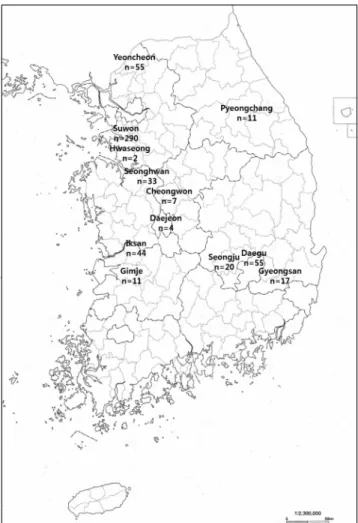
Finally, the FR data set and the data set containing generated climatic variables were combined into the final data set used for statistical analysis. Data points with missing values (n=75) were eliminated. Under the normality assumption, the outliers (n=8) were deleted after detection via box-plots. Therefore, a final data set (n=549) with DMY values of FR, 12 cultivated locations, and climatic variables was generated and used in the following analyses. As showed in Fig. 1, the 12 cultivated locations in the final data set were Gyeongsan (n=17), Gimje (n=11), Daegu (n=55), Daejeon (n=4), Seongju (n=20), Seonghwan (n=33), Suwon (n=290), Yeoncheon (n=55), Iksan (n=44), Cheongwon (n=7), Pyeongchang (n=11), and Hwaseong (n=2).
2. Analysis Method
1) Optimal climatic variables detection
Multiple regression analysis is a basic linear model used to assess the association between two or more continuous explanatory variables and a single continuous response variable (Mardia et al., 1979). The multiple regression equation is as follows:
Yn1Xn(p1)(p1)1n1, ~ i.i.d. N (0, ε δ2)
Where Y is the vector of the response variable, X is the vector of explanatory variables, β is the matrix of coefficients of explanatory variables, and ε is the vector of residual. ε is independent and identically distributed normal which have a mean (as 0) and a variance (as δ2). Both explanatory and response variables should be normally distributed.
Multicollinearity among explanatory variables was checked since more than 2 explanatory variables which had the same role were included in the model. Multicollinearity is a problem in which two or more predictor variables in a multiple regression model are strongly correlated and result in the inexistence of the inverse matrix ((XTX) 1) and subsequently the distortion of regression coefficient (Farrar et al., 1967).
There was a high possibility of multicollinearity in this multiple regression analysis for the reason that many
Fig. 1. Map with sample size of the 12 cultivated locations in the final data set.
climatic variables were included in reality. Therefore, the correlation coefficients were calculated through correlation analysis among all the response and explanatory variables.
Based on the variance inflation factor (VIF) and correlation coefficients, some variables with multicollinearity were eliminated to avoid the distortion due to the confounding effects in interpretation.
2) Final model construction through general linear model
General linear model was used for constructing the final model including the continuous climatic variables and cultivated locations as dummy variables. The general linear model in this research is as follows:
1 1 1
) 1 ( ) 1 (
1
n p p n c c n
n X Z
Y , ~ i.i.d. N (0, ε δ2)
Where Y is the vector of response variable, X is the vector of explanatory variables. β is the matrix of coefficients of explanatory variables, Z is the matrix of dummy variables (q = 4) γ is the matrix of coefficients of dummy variables and ε is the vector of residual. ε is independent and standard normally distributed under homogeneity. Dummy variable is indicator that takes 0 or 1. In this research, dummy variables (probable to express 24= 16 variables at maximum) were used to express the 12 cultivated locations. For instance, the dummy variables for Gyeongsan and Gimje were (1, 0, 0, 0) and (0, 1, 0, 0), respectively. Moreover, the last category which was Hwaseong, all the numerical values in the dummy variable were 0.
The final model was constructed via general linear model using the variables without multicollinearity and selected through multiple regression analysis by stepwise approach.
In the model, only the main effects of climatic variables and cultivated locations were included, which means the interaction effects were not considered.
3) Model diagnostic
Residual diagnostics was used to check the goodness- of-fit of the model. To check the relation between observed values and predicted values, standardized residuals of the final model were calculated. Then, Probability-Probability plot (P-P plot), scatter plot of standardized residuals against
predicted values, and the plot of 95% confidence interval were prepared to check the goodness-of-fit of the final model to the data set used in this research. For P-P plot, linear relation between observed values and predicted values indicates the model fit the data used in this research well under the normality assumption. Moreover, when the scatter plot of standardized residuals against the predicted values shows a pattern (for example: logarithm, exponential or quadratic shape), the model may not fit the data used in the research well. In other words, no pattern of standardized residuals means the model fit the data used in the study well. Furthermore, in the plot of 95% confidence interval, the fitness of the model to the data set used in the research could be well confirmed if most scatters fall into the 95% confidence interval.
All statistical analyses were performed using SPSS 21.0 (IBM Corp, 2012) in this study.
. RESULTS AND DISCUSSION
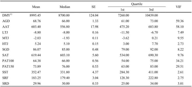
The descriptive statistics of all variables in this study were presented in Table 1. The mean of DMY was 8,995.45 (kg/ha) and the first quartile and the third quartile were 7,260.00 (kg/ha) and 10,439.00 (kg/ha), respectively. The mean and median were similar (8,995.45 vs. 8,700.00) and the differences between mean and the first and third quartile were similar (1,735.45 vs. 1,443.55). Therefore, it was judged that DMY was symmetrically distributed.
Meanwhile, other variables were also symmetrically distributed.
AGD, AAT, PAT100, and PAT150 were considered to have multicollinearity problems based on the results of detection of multicollinearity. In general, it was considered that multicollinearity is present when VIF is bigger than 10 (Allison, 1999). The reason for multicollinearity of AGD and AAT might be many temperature related variables was included as explanatory variables, and for the multicoll- inearity between PAT100 and PAT150, the reason might be they were both time related variables and had some repeated information.
To solve the multicollinearity problems, correlation analysis including all explanatory variables was performed and the correlation matrix was presented in Table 2. The strong correlations (correlation coefficient > 0.7) were observed
between AGD and AAT, SGD and SAT, LTJ and MTJ, PAT100 and PAT150. Due to the multicollinearity, AGD and PAT100 were eliminated. Therefore, the rest variables included AAT, LTJ, MTJ, HTJ, SGD, SAT, PAT150, SST, SRF, and SRD were used in multiple regression analysis.
As showed in Table 3, the optimal model was generated
using stepwise approach (a p-value less than 0.05 was considered) of multiple regression analysis, including the explanatory variables selected based on the results of multicollinearity and correlation analysis. The adjusted R square was 12.4% here (p < 0.01). In this model, the VIF of all the explanatory variables (AAT, SGD, PAT150, MTJ, Table 1. Descriptive statistics, normality, and multicollinearity diagnostics for all the explanatory variables
Mean Median SE Quartile
1st 3rd VIF
DMY1) 8995.45 8700.00 124.04 7260.00 10439.00
AGD 68.76 66.00 1.33 61.00 73.00 59.36
AAT 603.40 556.80 17.98 475.20 683.80 58.10
LTJ -8.80 -8.00 0.16 -11.50 -6.70 7.49
MTJ -2.03 -1.93 0.11 -3.62 0.21 9.55
HTJ 5.24 5.10 0.15 3.00 7.70 2.73
SGD 86.07 85.00 0.48 79.00 92.00 8.22
SAT 619.44 603.10 5.60 534.00 690.30 9.76
PAT100 64.38 66.00 0.56 54.00 75.00 34.21
PAT150 73.89 76.00 0.53 63.00 83.00 29.51
SST 352.47 331.80 4.37 284.30 411.00 2.61
SRF 183.25 179.40 3.04 128.30 222.80 2.75
SRD 29.96 30.00 0.33 25.00 34.00 3.01
1)DMY, dry matter yield; AGD, autumnal growing days; AAT, autumnal accumulated temperature; LTJ, lowest temperature in January;
MTJ, mean temperature in January; HTJ, highest temperature in January; SGD, spring rainfall days; SAT, spring accumulated temperature; PAT100, period to accumulated temperature 100; PAT150, period to accumulated temperature 150; SST, spring sunshine time; SRF, spring rainfall; SRD, spring rainfall days.
Table 2. Correlation matrix including all the explanatory variables
AGD AAT LTJ MTJ HTJ SGD SAT PAT100 PAT150 SST SRF SRD
AGD1) 1 .986** -.102* -.054 -.120** -.128** -.091* .126** .116** -.064 .021 .013
AAT 1 -.052 -.031 -.094* -.093* -.063 .119** .111** -.078 .034 .043
LTJ 1 .865** .452** .260** .097* -.480** -.474** .105* -.123** -.318**
MTJ 1 .674** .203** -.012 -.619** -.594** .008 -.014 -.226**
HTJ 1 .208** .006 -.628** -.613** -.037 .025 -.052
SGD 1 .871** -.406** -.392** .316** .245** .151**
SAT 1 -.154** -.159** .565** .184** .158**
PAT100 1 .980** .056 -.047 .256**
PAT150 1 .023 -.007 .261**
SST 1 -.281** -.146**
SRF 1 .692**
SRD 1
* p <0.05, ** p < 0.01
1)AGD, autumnal growing days; AAT, autumnal accumulated temperature; LTJ, lowest temperature in January; MTJ, mean temperature in January; HTJ, highest temperature in January; SGD, spring rainfall days; SAT, spring accumulated temperature; PAT100, period to accumulated temperature 100; PAT150, period to accumulated temperature 150; SST, spring sunshine time; SRF, spring rainfall; SRD, spring rainfall days.
SRF, and SRD) were less than 3 which means it could be concluded that there is no multicollinearity. Furthermore, the effects of explanatory variables in regressions could be recognized by checking the changing degrees of plus-minus signs and magnitudes of Pearson’s correlation coefficients, partial correlation coefficients, and part (semi partial) correlation coefficients of explanatory variables (Cohen et al., 2003). Here, the Pearson’s correlation coefficient is a statistic of the strength of a linear relationship between two variables (Hauke and Kossowski, 2011), partial correlation coefficient is designed to eliminate the effect of one variable on two other variables when assessing the correlation between these two variables, while part (semi partial) correlation coefficient is used to express the specific portion of variance explained by a given explanatory variable in a multiple regression analysis (Abdi, 2007).
AAT and SRD had no overlapping effects with other variables based on the results that the magnitudes of correlation coefficients were similar, this means it could be concluded that AAT and SRD were independent in principle. Therefore, the effects of AAT and SRD could be interpreted in the way that DMY will increase 1.401 and 55.390 respectively when these two variables increase 1 unit. Meanwhile, other variables might have overlapping effects with each other for the same reason, and the effects of these variables couldn’t be explained in the same way for the reason that they are not independent with each other.
Pearson’s correlation coefficient could be calculated to
investigate the effects of explanatory variables on the response variable. AAT had the biggest Pearson’s correlation coefficient which was 0.197, the Pearson’s correlation coefficients of the rest variables were shown as descending in the sequence of SGD, PAT150, MTJ, SRF, and SRD.
This means the variables related to the autumn and next spring had strong effects on the DMY in this data set. The growth and development of FR is active during autumn and the next spring, so early seeding in autumn is important for FR to live safely through the winter. Meanwhile, the FR yield could be ensured if seeding was done in the next spring when seeding period was missed in autumn (Lorenz, 1991).
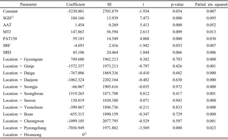
The cultivated locations were added in the form of dummy variables to general linear model with the selected climatic variables (AAT, SGD, PAT150, MTJ, SRF, and SRD). The result was presented in Table 4. The adjusted R square was 24.4% (p < 0.01). The adjusted R square was calculated as the partial eta squared because dummy variables were included in model. The FR dry matter yield estimation model based on climate data by locations in South Korea was as follows:
DMY = 104.166 SGD + 1.454 AAT + 147.863 MTJ + 59.183 PAT150 4.693 SRF + 45.106 SRD 5230.001 + Location
For a specific location, Location in the formula should be substituted by a constant value which was calculated for Table 3. Results of optimal stepwise multiple regression model for FR including climatic variables (R square
=.133**, adjusted R square = .124**)
Coefficient Standard
coefficient t p-value VIF Correlation coefficient
B SE Pearson’s Partial Part
Constant -1798.158 1525.401 -1.179 0.239
AAT1) 1.407 0.279 0.204 5.051 0.000 1.020 0.197 0.212 0.202
SGD 72.750 11.868 0.280 6.130 0.000 1.301 0.179 0.255 0.245
PAT150 52.241 13.000 0.223 4.019 0.000 1.926 0.081 0.170 0.161
MTJ 172.208 54.098 0.159 3.183 0.002 1.568 0.047 0.135 0.127
SRF -8.118 2.361 -0.199 -3.439 0.001 2.094 -0.026 -0.146 -0.138
SRD 55.390 22.867 0.147 2.422 0.016 2.289 0.082 0.103 0.097
1)AAT, autumnal accumulated temperature; SGD, spring growing days; PAT150, period to accumulated temperature 150; MTJ, mean temperature in January; SRF, spring rainfall; SRD, spring rainfall days.
this specific location as showed in Table 4. For instance, the FR dry matter yield estimation model of Gyeongsan would be DMY = 104.166SGD + 1.454AAT + 147.863MTJ + 59.183PAT150 4.693SRF + 45.106SRD 4480.321 after inputting the Location constant value 749.680. By comparing the results of Table 3 with 4, it was found that the regression coefficients of SRF and SGD had obvious changes by adding the location variable. This might indicate that SRF and SGD were not independent with location, which means SRF and SGD could reflect the distinct characteristics of different cultivated locations. Meanwhile, it was shown that there was no change in the coefficient of AAT. This was thought to be that farmers in different cultivated locations would adjust the seeding date in autumn to ensure FR receives enough accumulated temperature before winter. SGD had the biggest partial eta squared, the partial eta squared of the rest variables were shown as descending in the sequence of AAT, PAT150, MTJ, SRF
and SRD. This might indicate that growing days in spring has the biggest effect on DMY and subsequently accumulated temperature in autumn also had an important effect.
Therefore, attention should be paid to early enough seeding in autumn to ensure FR get enough accumulated temperature before winter, and enough growing days in next spring is also important for the growth of FR. The result that the effects of MTJ, SRF, and SRD were small may reflect the good cold tolerance and strong drought tolerance of FR.
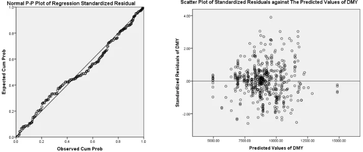
Fig. 2 presented the plots of residual diagnostic for assessing the goodness-of-fit of this model. The P-P plot is used for comparing the accumulated probability of DMY observations and the accumulated probability of predicted DMY values. In general, the points arranged on the line neatly shows that the normality assumption of the residual is satisfied. Here, the P-P plot of regression standardized residuals exhibited a fluctuation pattern around the 45- degree line; therefore future researches on adding curvilinear
Table 4. Results of general linear regression model for FR including selected climatic variables and cultivated locations (R square = .267**, adjusted R square = .244**)
Parameter Coefficient SE t p-value Partial eta squared
Constant -5230.001 2703.879 -1.934 0.054 0.007
SGD1) 104.166 13.939 7.473 0.000 0.095
AAT 1.454 0.269 5.413 0.000 0.052
MTJ 147.863 56.594 2.613 0.009 0.013
PAT150 59.183 14.549 4.068 0.000 0.030
SRF -4.693 2.416 -1.942 0.053 0.007
SRD 45.106 24.464 1.844 0.066 0.006
Location = Gyeongsan 749.680 1962.213 0.382 0.703 0.000
Location = Gimje -1572.357 1973.213 -0.797 0.426 0.001
Location = Daegu -767.006 1869.336 -0.410 0.682 0.000
Location = Daejeon -1062.324 2202.164 -0.482 0.630 0.000
Location = Seongju -66.067 1905.616 -0.035 0.972 0.000
Location = Seonghwan 1519.265 1871.708 0.812 0.417 0.001
Location = Suwon 130.819 1830.380 0.071 0.943 0.000
Location = Yeoncheon -399.867 1896.736 -0.211 0.833 0.000
Location = Iksan -655.315 1890.159 -0.347 0.729 0.000
Location = Cheongwon -1099.105 2077.795 -0.529 0.597 0.001
Location = Pyeongchang -7036.949 1971.882 -3.569 0.000 0.023
Location = Hwaseong 02)
1)SGD, spring growing days; AAT, autumnal accumulated temperature; MTJ, mean temperature in January; PAT150, period to accumulated temperature 150; SRF, spring rainfall; SRD, spring rainfall days.
2)This parameter is set to zero because it is redundant.
forms (quadratic or cubic form) of response variable to the model were necessary. Furthermore, the points were scattered well without a particular pattern on the figure of predicted values of DMY and standardized residuals of DMY, this means that the homoscedasticity and the assumption that the mean of the residuals are equal to zero were satisfied.
As presented in Fig. 3, though the contribution rate of this model is small, the fitness of the model is proper based on most scatters of the predicted DMY values fell in the 95% confidence interval. The low contribution rate of
this model could be explained by that many yield related variables were not included in this research.
Additionally, researches on interaction terms were also applied. Though the goodness-of-fit of the model turned a little better, it was difficult to interpret the effect of interaction terms. Therefore, the interaction terms were not included in the final model to for better predictability and simplicity of the model.
. CONCLUSION
In this study, a yield prediction model for FR using climatic variables by locations in Korea was constructed.
The results suggest that though the adjusted R square of this model was 24.4%, the goodness-of-fit and results of residual diagnostics were acceptable. In further researches, adding curvilinear forms of response variable and more yield related explanatory variables to the model were necessary to improve the adjusted R square.
. ACKNOWLEDGEMENT
This study was supported by a grant from the Bio- industry Technology Development Program (313020-04), Ministry of Agriculture, Food, and Rural Affairs, Republic of Korea and also with the support of the “Cooperative Research Program for Agriculture Science and Technology Fig. 2. Results of residual diagnosis (left: normal P-P plot of standardized residuals, right: scatter plot of
standardized residuals against predicted values of dry matter yield (DMY) from the model).
Fig. 3. Scatter plot including mean regression line and 95% confidence interval for observed dry matter yield and predicted dry matter yield from the model.
Development (Project No. PJ01028303),” Rural Development Administration, Republic of Korea.
. REFERRENCES
Abdi, H. 2007. Part (semi partial) and partial regression coefficients.
Encyclopedia of measurement and statistics. 736-740.
Ahn, J.H., Kim, K.D. and Lee, J.T. 2014. Growth Modeling of Chinese Cabbage in an Alpine Area. Korean Journal of Agricultural and Forest Meteorology. 16(4):309-315.
Allison, P.D. 1999. Multiple regression: A primer. Pine Forge Press, Newbury Park, CA, U.S.A. p142.
Bushuk, W. 1993. Rye Production and Uses Worldwide. In: R.
Macrae, R. K. Robinson, and M. J. Sadler (Ed.), Encyclopaedia of Food Science and Technology, vol. 6. Academic Press.
London. UK. pp. 3946-3950.
Cao, W. and Moss, D.N. 1997. Modelling phasic development in wheat: a conceptual integration of physiological components. The Journal of Agricultural Science. 129(2), 163-172.
Chang, J. and Clay, D.E. 2005. Identifying factors for corn yield prediction models and evaluating model selection methods.
Korean Journal of Crop Science. 50(4):268-275.
Cohen, J., Cohen, P., West, S.G. and Aiken, L.S. 2003. Applied multiple regression/correlation analysis for the behavioral sciences. Routledge, New York, U.S.A. pp. 310-316.
Dahikar, S.S. and Rode, S.V. 2014. Agricultural crop yield prediction using artificial neural network approach. International Journal of Innovative Research in Electrical, Electronics, Instrumentation and Control Engineering. 2(1):683-686.
Delgado, C.L. 2003. Rising consumption of meat and milk in developing countries has created a new food revolution. The journal of nutrition. 133(11):3907S-3910S.
Farrar, D.E. and Glauber, R.R. 1967. Multicollinearity in regression analysis: the problem revisited. The Review of Economic and Statistics. 92-107.
Harvey, M. and Pilgrim, S. 2011. The new competition for land:
food, energy, and climate change. Food Policy. 36:S40-S51.
Hauke, J. and Kossowski, T. 2011. Comparison of values of Pearson’s and Spearman's correlation coefficients on the same sets of data. Quaestiones geographicae. 30(2):87-93.
Huang, J. and Han, D. 2014. Meta-analysis of influential factors on crop yield estimation by remote sensing. International Journal of Remote Sensing. 35(6):2267-2295.
Johansson, D.J.A. and Azar, C. 2007. A scenario based analysis of land competition between food and bioenergy production in the US. Climatic Change. 82(3-4):267-291.
Kent, N.L. 1983. Rye and triticale. In: Technology of Cereals. 3rd ed. Pergamon Press, Oxford. pp.175-183.
Kim, K.D., Sung, K.I., Jung, J.I., Lee, E.J., Kim, E.J., Nejad, J.G., Jo, M.H. and Lim, Y.C. 2012. Suitability classes for Italian ryegrass (Loliummultiflorum Lam) using soil and climate digital database in Gangwon Province. The Korean Society of Grassland and Forage Science. 32(4), 437-446.
Kim, K.D., Sung, K.I., Joo, J.H., Kim, B.W., Peng, J.L., Lee, B.H., Nejad, J.G., Jo, M.H. and Lim, Y.C. 2013. Suitability Classes for Whole Crop Barley Using Soil and Climate Digital Database in Gangwon Province, Journal of Agricultural, Life and Environmental Sciences. 25(3), 26-31.
Kim, K.D., Suh, J.T., Lee, J.N., Yoo, D.L., Kwon, M. and Hong, S.C. 2015. Evaluation of factors related to productivity and yield estimation based on growth characteristics and growing degree days in highland Kimchi cabbage. Korean Journal of Horticultural Science & Technology. 33(6):911-922.
Kim, M.R. and Kim, S.G. 2014. Examining Impact of Weather Factors on Apple Yield. Korean Journal of Agricultural and Forest Meteorology. 16(4):274-284.
Kim, S.Y., Park, C.K., Gwon, H. S., Khan, M. I., and Kim, P. J.
2015. Optimizing the harvesting stage of rye as a green manure to maximize nutrient production and to minimize methane production in mono-rice paddies. Science of the Total Environment. 537:441-446.
Kryvobok, O. 2000. Estimation on the productivity parameters on wheat crops using high resolution satellite data. International Archives of Photogrammetry and Remote Sensing. 33(B7/2;
PART 7): 717-722.
Lee, H. and Moon, A. 2014. Development of yield prediction system based on real-time agricultural meteorological information.
Proceedings of 16th International Conference on Advanced Communication Technology. IEEE. 1292-1295.
Lee, S.G., Seo, T.C., Jang, Y.A., Lee, J.G., Nam, C.W., Choi, C.S., Yeo, K.H. and Um, Y.C. 2012. Prediction of Chinese cabbage yield as affected by planting date and nitrogen fertilization for spring production. Journal of Bio-Environment Control. 21(3), 271-275.
Lorenz, K.J. 1991. Rye. In: K. J. Lorenz and K. Kulp (Ed.), Handbook of Cereal Science and Technology. Marcel Dekker, New York, U.S.A. pp.331-371.
Na, S.I., Lee, K.D., Baek, S.C. and Hong, S.Y. 2015. Estimation of Chinese Cabbage Growth by RapidEye Imagery and Field Investigation Data. Korean Journal of Soil Science and Fertilizer.
48(5):556-563.
IPCC, 2007. Climate Change 2007: Impacts, Adaptation and
Vulnerability. Contribution of Working Group II to the Fourth Assessment Report of the Intergovernmental Panel on Climate Change. M.L. Parry, O.F. Canziani, J.P. Palutikof, P.J. van der Linden and C.E. Hanson, (Ed.), Cambridge University Press, Cambridge, UK, 976pp.
Peng, J.L., Kim, M.J., Kim, Y.J., Jo, M.H., Nejad, J.G., Lee, B.H., Ji, D.H., Kim, J.Y., Oh, S.M., Kim, B.W., Kim, K.D., So, M.J., Park, H.S. and Sung, K.I. 2015. Detecting the Climate Factors related to Dry Matter Yield of Whole Crop Maize. Korean Journal of Agricultural and Forest Meteorology. 17(3):261-269.
Rathmann, R., Szklo, A. and Schaeffer, R. 2010. Land use competition for production of food and liquid biofuels: An analysis of the arguments in the current debate. Renewable Energy. 35(1):14-22.
Schlenker, W. and Roberts, M.J. 2006. Estimating the Impact of Climate Change on Crop Yield: The Importance of Non Linear
Temperature Effects. No. w13799. National Bureau of Economic Research, 2008.
SPSS (2012). IBM SPSS Statistics 21.0. IBM Corp., Somers, New York. U.S.A.
Takahashi, S. 2002. A Model Predicting Forage Maize Growth Based on Temperature and Solar Radiation. Grassland Science. 48(1), 43-49.
Yun, J.I. 2003. Predicting regional rice production in South Korea using spatial data and crop-growth modeling. Agricultural Systems. 77(1):23-38.
Zhang, H., Chen, H. and Zhou, G. 2012. The model of wheat yield forecast based on modis-ndvi: a case study of Xinxiang.
Proceedings of the ISPRS Annals of the Photogrammetry, Remote Sensing and Spatial Information Sciences Congress.
(Received July 4, 2016 / Revised July 23, 2016 / Accepted August 4, 2016)