Validations of a Numerical Model of Solute Transport in a Snowpack

전체 글

(1)자원환경지질, 제45권, 제5호, 525-533, 2012 Econ. Environ. Geol., 45(5), 525-533, 2012. Validations of a Numerical Model of Solute Transport in a Snowpack Jeonghoon Lee* Korea Polar Research Institute, Incheon, 406-840, Korea. 눈 속에서 용질이동을 모사하기 위한 수치모델의 검증 이 정 훈* 극지연구소, 극지지구시스템연구부 겨울철동안 쌓여 봄에 놓은 눈 녹은 물(snowmelt), 즉 융설의 유출은 북반구 및 산간지역에서 매우 중요한 것으로 여 겨지고 있다. 이러한 지역에서 융설로 인한 유동 및 이온의 이동에 대한 이해는 매우 중요하며 전세계적으로 꾸준하게 연구되고 있다. Lee et al. (2008a)와 Lee et al. (2008b)연구에서는 대기로부터 수송된 이온 및 오염원이 융설에 의해 눈 속을 이동하는 것을 모사하기 위한 Mobile-Immobile water Model (MIM)을 개발하였다. 이 연구에 사용된 모델을 검증 하기 위해서 물질수지계산(mass balance calculation) 및 해석해(analytical solution)를 이용한 모델결과와의 비교를 수행하 였다. 일정시간동안 눈 속에서의 물질의 질량변화는 눈 표면에서 들어온 물질과 눈 기저부에서 빠져나간 물질의 질량 차 이와 같아야한다는 사실을 이용하여 물질수지를 계산하였다. 파면(wave front)의 이동속도 및 기존문헌에서 알려진 해석 해를 이용하여 모델결과와의 비교도 시도하였다. 모델의 물질수지계산결과 질량 차이가 거의 발생하지 않았으며 모델결 과와 해석해와의 비교 역시 두 결과가 거의 일치하였다. 주요어 : 융설, Mobile-Immobile Model, 물질수지계산. Snowmelt from seasonal snow covers can be significant in many environments of northern and alpine areas. Water flow and chemical transport resulting from snowmelt have been studied for an understanding of contributions to watersheds or catchments. A Mobile-Immobile water Model (MIM) was developed to describe the movement of ionic tracers through a snowpack by Lee et al. (2008a) and Lee et al. (2008b). To validate the model used in the studies, mass balance calculations of the model were conducted and comparisons were made between model results and analytical solutions in this work. Mass balance was calculated based on the fact that change in total mass within a snowpack with time is equal to sum of any change in the flux of water or ionic tracers into and out of the snowpack. Calculations of both water and ionic mass show almost perfect agreement between changes of two water and solute mass fluxes. Comparisons between model results and analytical solutions including wave velocity and effective saturation show almost perfect agreement. Key words : snowmelt, Mobile-Immobile Model, mass balance calculation. 1. Introduction. through melting processes. This winter storage and spring release of precipitated water has important consequences for the water resources of catchments in many alpine areas (Meixner et al., 2004). Seasonal snow supplies to water reservoirs and recharges groundwater aquifers during spring. Therefore, snowmelt is a major component of the hydrological cycle in many regions and is an important consideration for water resourses (Singh et al., 1997).. Precipitation is of major interest in the water cycle, and is the ultimate source of water to catchments or watersheds. Seasonal snow covers over 25% of the Earth’s land surface, distributing mostly at high latitude and at high altitude areas (Rodhe, 1998). This stored water of precipitation in snowpack greatly affects the hydrological regime *Corresponding author: [email protected]. 525.

(2) 526. Jeonghoon Lee. Seasonal snow covers can be significant in the chemical dynamics of ecosystems in many regions. For example, terrestrial nitrogen export (N) during snowmelt to aquatic ecosystems is linked to nitrogen saturation and freshwater acidification. An exponential decrease of solute concentration (i.e., an ionic pulse) has been reported through the melting season and so have diurnal variations that were negatively related to the melting rate (Lee et al., 2008a). The solutes tend to leave the snowpack with the first meltwater, which may be much higher in solutes than the original snowfall during snow metamorphism or snow redistributions, which causes low pH values in the streams with health hazards for the biota (Williams et al., 1995). Hibberd (1984) simulated the ionic pulse using a standard advection-dispersion model, which was unable to simulate the long-tail following initial solute arrival. This limitation was improved by a mobile-immobile model (MIM), which provided one simple conceptualization for modeling preferential flow in snow (Harrington and Bales, 1998). In the MIM, solutes in the mobile water are transported by advection and dispersion, and those in the immobile water are transported only by exchange between immobile and mobile water (Harrington and Bales, 1998; Feng et al., 2001; Lee et al., 2008a). In early model (e.g., Harrington and Bales, 1998), the exchange between mobile and immobile water was parameterized by first order kinetics with an invariant exchange rate constant. Feng et al. (2001) discovered that an invariant exchange rate constant cannot explain their observed results in a rain-on-snow experiment, in which tracer concentrations positively associated with the input flux. Lee et al. (2008b) monitored chemical compositions of both natural and artificial tracers flowing fresh snow, snow profile and snowmelt. They observed that natural tracers showed negative concentration-discharge relationship while artificial tracers showed positive relationship under same hydrological condition. To better understand how hydrological conditions control solute transport and redistribution in a snowpack, it is, however, limited to use the model by Feng et al. (2001) to simulate both types of concentration-discharge relationship with a common set of hydrological parameters. Lee et al. (2008a) described artificial rain-on-snow experiments onto. a snowpack to understand how hydrological and chemical conditions cause a positive or negative relationship between meltwater in discharge and solute concentration based on observations from the experiments and those of Feng et al. (2001). Lee et al. (2008a) tested the necessity of having a flow-dependent exchange rate coefficient as proposed by Feng et al. (2001) under different hydrological and chemical conditions for simulating both the positive and negative concentration-discharge relationships using the MIM. Here we present a validation of the MIM used by Lee et al. (2008a) and Lee et al. (2008b), which has never been discussed elsewhere. Our objective in doing this is to develop and validate the capability to investigate the solute transport in a snowpack, and thence to use this model to explore concentration-discharge relationships under various hydrological and chemical conditions. In this paper, we first describe how to validate the model and then compare results from the model with analytical solutions and mass balance calculations.. 2. Theoretical Background Both flow and transport model can be verified using mass balance and analytical solutions. Change in total mass within snowpack with time is equal to sum of any change in the flux of water or ionic tracers into and out of snowpack. For flow model, we can compare the wave front velocity at the surface under a certain circumstance. On the other hand, van Genuchten and Wierenga (1976) derived analytical solution for mobile and immobile water exchange. The analytical solution will be used to verify the accuracy of mobile and immobile model (MIM) presented here. The variables used in these and following equations are described in Table 1. 2.1. Mass balance As introduced earlier, Eq. (1) describes that total water mass change within the snowpack with time is equal to sum of any changes in the flux n ( q = ρKS ) of water and ice into and out of snowpack. z=bottom. z=bottom. ∫z=surface (a + b)t=t dz – ∫z=surface (a + b)t=t dz 1. =∫. t=t2. t=t1. n. 2. n. [ (ρKS )z=surface – (ρKS ) z=bottom]dt. (1).

(3) Validations of a Numerical Model of Solute Transport in a Snowpack. 527. Table 1. Snowpack properties and symbols used in this study Meaning (Values used in the simulations if not otherwise specified) α αi αm b Ci Cice Cm Cr D d g K k n qz S. total mass of water per unit snow volume mass of immobile water per unit snow volume mass of mobile water per unit snow volume mass of ice per unit snow volume tracer concentration in immobile phase initial concentration in ice (Cice = 0) tracer concentration in mobile phase tracer concentration when sprayed dispersion coefficient dynamic dispersivity (d = 0.05) gravitational acceleration hydraulic conductivity intrinsic permeability exponent specific discharge effective water saturation (Sw − Si)/(1 − Si). Si. irreducible water content: irreducible volume of water over pore volume total water content: total water volume over the pore volume time water velocity melting rate spraying rainfall rate depth (z = 200) Si/(1 − Si) volumetric water content density of ice density of water porosity exchange rate coefficient. Sw t u Vmelt Vrf z β θ ρice ρw φ ω. where K is saturated hydraulic conductivity, S is effective saturation, n is empirical exponent, a is the mass of water and b is the mass of ice per unit snow volume, z is the depth into the snowpack, t is time and ρ is the density of water. 2.2. Analytical Solutions for Flow 2.2.1. Wave velocity The model can be verified using the wave velocity. When there is a discontinuity of water content (wave front) in the snowpack, the position of wave front can be determined by the wave velocity, Vs (Hibberd, 1984; Feng et al., 2001),. Units. Dimension -3. g cm g cm-3 g cm-3 g cm-3 g/cm-3 g/cm-3 g/cm-3 g/cm-3 cm2/h cm cm h-2 cm h-1 cm2 cm h-1. g g g g g. of of of of of. total water/ cm3snow immobile water/ cm3snow mobile water/ cm3snow ice/ cm3snow solute mass/cm3ofimmobilewater. g of solute mass/cm3ofmobilewater g of solute mass/cm3ofwater. 3 qz = KS3 cm of snow*cm3water/(cm3snow*h) cm3of(totalwater-immobile) volume / cm3 of (pore-immobile) volume cm3ofimmobilewatervolume/cm3 of pore volume cm3oftotalwatervolume/cm3 of pore volume. h cm h-1 cm h-1 cm h-1 cm. -3. g cm g cm-3. cm snow/s cm3ofsnowvolume/(cm2 of snow*h) cm3ofwatervolume/(cm2 of snow*h). cm-3ofwatervolume/cm3 of pore volume g of ice/ cm3ofice g of water/ cm3ofwater cm-3ofporevolume/cm3 of total volume. h-1. n. n. K S + – S– Vs = -------------------------------φ ( 1 – Si ) S + – S–. (2). where the subscripts plus and minus represent values directly behind and preceding the wave front, φ is the porosity, Si is irreducible water content in the snowpack and S is the effective water saturation. 2.2.2. Solutions of S When two wave fronts move through the snowpack, water content (S) between two wave.

(4) 528. Jeonghoon Lee. front that have different water content (S1, S2) can be presented in literature (Feng et al., 2001) as following, z S = ---------------n ( t – t2 ). 1 --------n–1. (3). This solution can be applied when S2 is less than S1, which means a sudden decrease of water content at the surface. t2 is when the water content changes at the surface. One-dimensional water percolation in snow is as following, n. ∂S ∂(KS ) φ (1 – Si)------ + ---------------- = 0 ∂t ∂z. (4). 2.3. Analytical solutions for transport 2.3.1. Solutions of Cm van Genuchten and Wierenga (1976) developed a mathematical model to describe the chemical transport. The following general system of equations (Eqs. 4 to 8) depicts the mobile and immobile phases, resulting from a pulse input of solute. 2. ∂C ∂Cim ∂C ∂C - = θmD-----------m – vmθm---------m θm---------m + θim---------2 ∂t ∂t ∂z ∂z. (5). ∂Cim - = α(Cm – Cim) θim---------∂t. (6). ∂C ⎧ vm C0 0 ≤ T < T 1 lim+ vmCm – D---------m = ⎨ z→0 ∂z T ≥ T1 ⎩ 0. (7). lim [ Cm(z,t)] = 0. (8). Cm(z,0) = Cim(z,0) = 0. (9). z→∞. where θm and θim are mobile and immobile water content, respectively, vm is average pore-water velocity in dynamic region, D is dispersion coefficient and α is mass transfer coefficient. The following analytical solutions were presented for the relative concentrations in the mobile and immobile liquids in van Genuchten and Wierenga (1976). 0 ≤ T < T1 c1(x,T) ⎧ cm(x,T) = ⎨ ⎩ c1(x,T) – c1(x,T – T1) T ≥ T1. (10). c2(x,T) 0 ≤ T < T1 ⎧ cim(x,T) = ⎨ ⎩ c2(x,T) – c2(x,T – T1) T ≥ T1. (11). αT c1(x,T) = G(x,T)exp(–αT ⁄ β) + ---∫G(x,τ)H1(T,τ)dτ R0. (12). T. c2(x,T) = α∫G(x,τ)H2(T,τ)dτ. (13). 0. 1 1⁄2 G(x,T) = ---erfc{(P ⁄ 4βT) (βx – T)} 2 1⁄2 1 –---(1 + Px + PT ⁄ β)exp(Px)erfc{(P ⁄ 4βT) (βx + T)} 2 1⁄2 2 (14) +(PT ⁄ πβ) exp{–P(βx – T) ⁄ 4βT} 1⁄2. H1(T,τ) = exp(–u–v){I0(ξ) ⁄ β + I1(ξ)(u ⁄ v) ⁄ (1 – β)}. (15) 1⁄2. H2(T,τ) = exp(–u–v){I0(ξ) ⁄ (1–β) + I1(ξ)(v ⁄ u) ⁄ β}. (16) u = ατ ⁄ β. (17). v = α(T – τ) ⁄ (1 – β)R. (18). ξ = 2(uv). 1⁄2. (19). where cm and cim are relative concentrations of mobile and immobile water, respectively, β = φRm/R, R is average retardation factor, and I0 and I1 are modified Bessel functions of the second kind of 0 and 1. 2.3.2. Wave velocity The chemical composition of wave front can be derived in Feng et al (2001). So the position of wave front is determined by the wave velocity, Vc + n. –. n. +. –. ∂C ∂C K Cm S+ – C m S– Vc = ---------------------------------------------- – S+D+---------m- + S– D– ---------m+ – φ ( 1 – Si ) C S – C S ∂z ∂z m + m –. (20) In this model, water that percolates through the snowpack can be from rainfall and snowmelt. Therefore mass balance calculations and analytical.

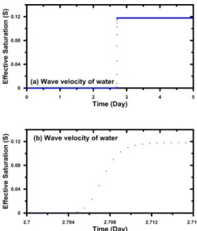
(5) Validations of a Numerical Model of Solute Transport in a Snowpack. solutions are divided into part of rainfall and snowmelt.. 3. Model Verification 3.1. Rainfall 3.1.1. Mass balance calculation The snowpack properties and modeling parameters were described in Lee et al. (2008a). The initial condition of snowpack is dry (S=0). Rainfall was applied 2.5 days later and the rainfall rate was 3 cm/hr. Figs. 1 and 2 show mass balance calculation of water and solute caused by the rainfall. The snowpack has a constant thickness. There is a sudden increase of water mass right after 2.5 days. When the rainfall is applied, the water mass in the snowpack increases so that the two changes show positive values. It shows almost perfect agreement between change of water mass in the snowpack and change of water flux. Discrepancy between change of water mass in the snowpack (14.994 g/cm2) and change of water flux (15.003 g/cm2) is 0.06% of the change of water flux (Fig. 1). Total mass change of ionic tracer within the snowpack (149.9 g/cm2) with time is equal to sum of any changes in the flux of ionic tracer into and out of snowpack (150.01 g/cm2). It also shows almost perfect agreement between changes of two solute mass fluxes (Fig. 2). The error is 0.07% of the change of. Fig. 1. Mass balance calculation for water only considering rainfall.. 529. solute flux. 3.1.2. Wave velocity Eqs. (2) and (19) describe water and chemical wave velocities. First, water wave velocity in Eq. (2) is 40 cm/hr and it takes 5 hours for water front to reach at the bottom, theoretically. Therefore, the wave front will be at the bottom after 0.208 days. Fig. 2. Mass balance calculation for solute by rainfall.. Fig. 3. Water wave front velocity calculation by rainfall..

(6) 530. Jeonghoon Lee. Fig. 5. Mass balance calculation of water caused by snowmelt.. Fig. 4. Chemical wave front calculation by rainfall.. because of the change of water saturation at the surface. The rainfall was applied after 2.5 days, so we can observe the wave front 2.708 days later at the bottom. This agrees well with the model calculation (Fig. 3). Using chemical wave velocity in Eq. (20), chemical wave velocity is 40.01 cm/hr and it takes 0.207 day for chemical front to be at the bottom. So we can observe the wave front 2.707 days later at the bottom. This also agrees well with the model calculation (Fig. 4). 3.2. Snowmelt 3.2.1. Mass balance calculation Figs. 5 and 6 show mass balance calculation of water and solute only due to snowmelt. The water mass in the snowpack decreases because it loses water mass when snow melts. In Fig. 5, it shows perfect agreement between change of water mass in the snowpack (–5.478 g/cm2) and change of water flux (–5.4874 g/cm2). Mass balance error between two changes of water is 0.17%. Total mass change of ionic tracer within the snowpack (–317.43 g/cm2) with time is equal to sum of any changes in the flux of ionic tracer into and out of snowpack (–316.42 g/cm2). It also shows almost perfect agreement between changes of two solute. Fig. 6. Mass balance calculation of solute by snowmelt.. mass fluxes. The error is 0.32% of the change of solute flux (Fig. 6). 2.2.2 Wave velocity Figs. 7 and 8 show the wave front position calculated by model. As discussed earlier, Eqs. (2) and (20) confirm the wave velocity. Two equations results in 1.286 days and 3.593 days for each wave front to reach at the bottom. Like rainfall, calculations of wave velocity by snowmelt agree well with model calculations..

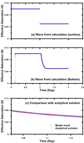
(7) Validations of a Numerical Model of Solute Transport in a Snowpack. 531. Fig. 7. Water wave front calculation by snowmelt.. Fig. 9. Comparison with analytical solutions.. solutions suggested by van Genuchten and Wierenga (1976) will be also examined. 4.1. Wave front calculation Eq. (3) predicts the effective water saturation at the bottom when boundary condition at the surface is changed, especially decrease of water content. The hydrological boundary condition at the snow surface equals the flux of water introduced to the snowpack as both rain and snowmelt (Lee et al., 2008a; Lee and Ko, 2011), n. Fig. 8. Chemical wave front calculation by snowmelt.. KSsurface ρw = Vrf ρw + (a + b)Vmelt. 4. Examples. = Vrf ρw + Vmelt[ φ (1 – Si)(Ssurface + β)ρw + (1 – φ )ρice] (21). There are two examples will be concerned to verify the MIM. First, flow part will be examined using Eq. (3). As discussed earlier, the analytical. where β = Si ⁄ (1 – Si) and ρice is the density of ice. Here, as suggested Feng et al. (2001), boundary condition (effective saturation, S) at the surface.

(8) 532. Jeonghoon Lee. will be changed from 0.1 to 0.05. Fig. 9 (a) shows that the effective saturation changed from 0.1 to 0.05 at the surface. Fig. 9 (b) shows the effective saturation at the bottom. Fig. 9 (c) shows comparison between model result (Eq. 4) and analytical solutions of effective saturation at the bottom for a certain period. The model results agree well with the analytical solution. 4.2 Analytical solutions for Cm Eqs. (5) to (19) describe mathematical governing equations (Eqs. 5 to 9) and semi-analytical solutions (Eqs. 10 to 19) for mobile and immobile model that needs some assumptions. Fig. 10 shows comparison between model results and analytical solutions, especially changing with exchange rate coefficient between mobile and immobile phases (α=0 and 0.15). Feng et al. (2001) and Lee et al. (2008) confirmed that it is necessary for the exchange coefficient to increase with water velocity for the solute transport in a snowpack. The numerical calculations by the governing equations agree well. with the analytical solutions suggested by van Genuchten and Wierenga (1976).. 5. Summary A Mobile-Immobile water Model (MIM) was developed to describe the movement of ionic tracers through a snowpack by Lee et al. (2008a) and Lee et al. (2008b). In this work, we have validated the model using mass balance calculations and analytical solutions. Mass balances of both water and ion were calculated based on the fact that change in total mass within a snowpack with time is equal to sum of any change in the flux of water or ionic tracers into and out of the snowpack. Calculations of both water and ionic mass show almost perfect agreement between changes of two water and solute mass fluxes. Comparisons were made between model results and analytical solutions including wave velocity and effective saturation and show almost perfect agreement. Chemical composition of a snowpack and its meltwater has never been investigated in Korea. Snowmelt-dominated systems in spring, for example, Jeju island and Ulleung island, should be studied to secure alternative water resources using snow chemistry. This work would be helpful to predict the chemical characteristics of a snowpack and its melt in those islands.. Acknowledgements This work was supported by KOPRI research grants (PE12070 and PE12110). Inputs from Dr. Feng and Dr. Posmentier at Dartmouth College significantly improved the quality of the paper. We appreciate two anonymous reviewers whose comments led to significant improvements.. References. Fig. 10. Comparison with analytical solution.. Feng, X., Kirchner, J.W., Renshaw, C.E., Osterhuber, R.S., Klaue, B. and Taylor, S. (2001) A study of solute transport mechanisms using rare earth element tracers and artificial rainstorms on snow. Water Resources Research, v.37, p.1425-1435. Harrington, R. and Bales, R.C. (1998) Modeling ionic solute transport in melting snow. Water Resources Research, v.34, p.1727-1736. Hibberd, S. (1984) A model for pollutant concentrations.

(9) Validations of a Numerical Model of Solute Transport in a Snowpack during snow-melt. Journal of Glaciology, v.30, p.58-65. Lee, J., Feng, X., Posmentier, E.S., Faiia, A.M., Osterhuber, R. and Kirchner, J.W. (2008a) Modeling of solute transport in snow using conservative tracers and artificial rain-on-snow experiments. Water Resources Research, v.44, W02411, doi:10.1029/2006WR005477. Lee, J. and Ko, K.S. (2011) An energy budget algorithm for a snowpack-snowmelt calculation. Journal of Soil and Groundwater Environment, v.16, p.82-89. Lee, J., Nez, V.E., Feng, X., Kirchner, J.W., Osterhuber, R. and Renshaw, C.E. (2008b) A study of solute redistribution and transport in seasonal snowpack using natural and artificial tracers. Journal of Hydrology, v.357, p.243-254. Meixner, T., Gutmann, C., Bales, R., Leydecker, A., Sickman, J., Melack, J. and McConnell, J. (2004) Multidecadal hydrochemical response of a Sierra Nevada watershed: sensitivity to weathering rate and changes in deposition. Journal of Hydrology, v.285, p.272-285. Rodhe, A. (1998) Snowmelt-Dominated Systems, In: Kendall, C., McDonnell, J.J. (Eds), Isotope Tracers in. 533. Catchment Hydrology, Elservier, Amsterdam, p.391433. Singh, P., Spitzbart, G., Hübl, H. and Weinmeister, H.W. (1997) Hydrological response of snowpack under rainon-snow events: a field study. Journal of Hydrology, v.202, p.1-20. van Genuchten, M.T. and Wierenga, P.J. (1976) Mass transfer studies in sorbing porous media: I. Analytical solution. Soil Science Society of America Journal, v.40, p.473-480. Wankiewicz, A. (1978) A review of water movement in snow, in Modeling of Snow Runoff, edited by S.C. Colbeck and M. Ray, p.222-252, U.S. Army Cold Region Research and Engineering Laboratory, Hanover, NH. Williams, M.W., Bales, R.C., Brown, A.D. and Melack, J.M. (1995) Fluxes and transformations of nitrogen in a high-elevation catchment, Sierra Nevada. Biogeochemistry, v.28, p.1-31. 2012년 8월 6일 원고접수, 2012년 10월 23일 게재승인.

(10)