http://dx.doi.org/10.23895/kdijep.2018.40.3.1
1
The Effect of Enhancing Unemployment Benefits in Korea:
Wage Replacement Rate vs. Maximum Benefit Duration
†By JIWOON KIM
*
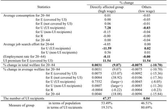
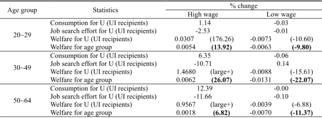
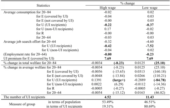
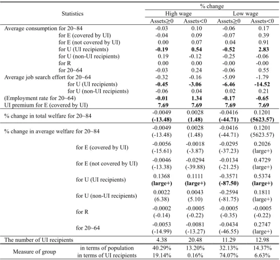
This paper studies the macroeconomic effects of an enhancement in unemployment benefits in Korea. In particular, I quantify the welfare effect of two specific policy chances which have been mainly discussed among policymakers in recent years: increasing wage replacement rates by 10%p and extending maximum benefit durations by one month. To this end, I build and calibrate an overlapping generation model which reflects the heterogeneity of the unemployed and the specificity of the unemployment insurance (UI) system in Korea. The quantitative analysis conducted here shows that extending maximum benefit durations by one month improves social welfare, whereas increasing wage replacement rates by 10%p deteriorates social welfare. Extending maximum benefit durations is applied to potentially all the UI recipients, including unemployed workers whose wage before job loss is relatively low and whose marginal utility is relatively high. However, increasing wage replacement rates is applied to only a small number of UI recipients whose wage before job loss is relatively high, while the increase in the UI premium is passed onto all of the employed. This study suggests that given the current UI system and economic environment in Korea, it is more desirable to extend maximum benefit durations rather than to increase wage replacement rates in terms of social welfare.
Key Word: Unemployment Insurance, Unemployment Benefits, Wage Raplacement Rate, Maximum Benefit Duration JEL Code: E24, J64, J65
I. Introduction
he unemployment insurance (UI) system is becoming increasingly important as the unemployment rate is expected to increase given that the restructuring of Korea's main industries (shipbuilding, construction, steel industry, etc.) is ongoing
* Fellow, Korea Development Institute (e-mail: [email protected])
* Received: 2018. 5. 10
* Referee Process Started: 2018. 5. 14
* Referee Reports Completed: 2018. 7. 31
† This paper is a revised and developed version of Kim (2016) and Kim (2017).
T
and the dynamics of the Korean economy are need to be restored. Moreover, there has been a constant discussion that Korea’s UI system has lower wage replacement rates and shorter maximum benefit durations as compared to those of other OECD nations. The wage replacement rate is 50.5%, lower than the OECD average (64.5%) while the maximum benefit duration is seven months on average, amounting to only half of the OECD average of 15.1 months. In this situation, there is growing recognition that unemployment benefits1 should be enhanced in Korea among policymakers and researchers. This paper investigates the macroeconomic effects of enhancing unemployment benefits in Korea using the overlapping generation model, which reflects the heterogeneity of the unemployed and the details of the UI system in Korea. In particular, I focus on two specific policy chances which have been mainly discussed among policymakers in recent years: increasing wage replacement rates by 10%p and extending maximum benefit durations by one month. I quantify the effect of these policy changes on aggregate consumption, the employment rate, and social welfare using the calibrated overlapping generation model.
Government support is needed for unemployment because unemployment is type of unexpected income shock, whereas there is no appropriate private insurance for unemployment risk due to the adverse selection problem. Consumption reduction resulting from unemployment not only reduces the welfare of the individual but also reduces the aggregate demand of the economy as a whole. Therefore, the government provides short-term income support on the premise of active job-seeking
WAGE REPLACEMENT RATES IN 2014(%) MAXIMUM BENEFIT DURATIONS IN 2010(MONTHS)
FIGURE 1.INTERNATIONAL COMPARISON OF UNEMPLOYMENT BENEFITS
Note: 1) Wage replacement rates specify monthly after-tax wage replacement (unemployment benefit amount/average monthly wage) for the first month of benefit receipt. 2) Comparisons of recipients aged 40 with long and uninterrupted employment records. 3) The OECD average indicates the average of the OECD nations shown in the graphs. 4) It should be noted that Belgium imposes no limits on duration. Therefore, the OECD average does not include the value for Belgium.
Source: Calculated by the author using OECD statistics and OECD (2011b).
1In this paper, the terms ‘unemployment insurance’ and ‘unemployment benefits’ are interchangeable.
0 10 20 30 40 50 60 70 80 90 100
U.K. Greece Poland U.S. Korea Turkey Sweden Ireland Estonia Austria Hungary Japan OECD average Slovakia Czech Germany France Spain Norway Iceland Italy Canada Netherlands Denmark Finland Portugal Belgium Slovenia Switzerland Luxembourg 0 5 10 15 20 25 30 35 40 45
Czech Slovakia U.S. U.K. Korea Italy Japan Austria Hungary Slovenia Turkey Canada Estonia Germany Greece Ireland Luxembourg Poland OECD average Switzerland Netherlands Finland Denmark France Norway Portugal Spain Sweden Iceland Belgium
through UI that serves as public insurance. The enhanced unemployment benefits can help the unemployed to maintain their consumption level and promote social welfare (consumption smoothing effects). However, more generous unemployment benefits can also have a negative impact on job search efforts (moral hazard effects). In addition, enhanced unemployment benefits potentially raise the UI premium for all workers. Therefore, when analyzing the effects of UI policy changes, it is necessary to reflect the effects on social welfare in a balanced manner in consideration of the positive aspects (consumption smoothing effects) and the negative aspect (moral hazard effects and the increase in the UI premium) of enhanced unemployment benefits.
In order to quantify the comprehensive effects of policy changes, I build an overlapping generation model which reflects the specificity of the UI system in Korea. In Korea, as of 2015, unemployment benefits are provided to involuntarily unemployed workers who have been in insurance-covered employment for at least 180 days during an 18-month period before their job loss. They are given 50% of the average daily wage before severance for terms of 90 to 240 days. The maximum benefit duration varies depending on the age and number of insurance- covered days of the worker (insured periods). The upper limit of the daily wage was set to 86,000 won, meaning that the upper limit of daily unemployment benefits is 43,000 won while the lower limit is 40,176 won—90% of the daily minimum wage (minimum wage × 8 hours).2
The novel feature of the model in this paper is that it incorporates upper and lower limits of unemployment benefits and the maximum benefit duration depending on the age and insured period of each worker into the overlapping generation model. In addition, the eligibility conditions for unemployment benefits (involuntary unemployment and the minimum insured periods) are explicitly reflected in the model. Lastly, the model includes both workers who are covered by the UI and those who are not. As mentioned above, the application of unemployment benefits depends on the age and wage level immediately before the job loss. In addition, the effects of policy changes in the UI system are likely to vary among the unemployed given their different characteristics, such as different ages, income levels, and amounts of net assets. Therefore, the model reflects the heterogeneity of workers in terms of age, individual productivity, and the amount of net assets.
The model is calibrated to match the key features of the Korean labor market, including labor market status by age group and various statistics related to the UI.
Using the calibrated model, the overall effects of enhanced unemployment benefits in Korea are examined. In particular, this paper focuses on two specific policy chances: increasing wage replacement rates by 10%p and extending maximum durations by one month. These two polices are compared because they are currently being discussed as feasible policy options to enhance unemployment benefits considering the current actual situation in Korea, whereas the effects of the two policy changes differ greatly. Because the range of the unemployed workers who will be affected by the policy change differs considerably between the two
2Minimum wages have rapidly increased over the past few years, even creating an inversion between the upper and lower limits in 2016. This was corrected recently via a revision of the Enforcement Decree of the Unemployment Insurance Act.
policy changes, the relative sizes of the consumption smoothing effects and moral hazard effects can also be very different. In addition, because the increases in the UI premium to achieve the two policy options differ, all workers who are paying or will pay the UI premium can be affected to some extent. In sum, the two policy options affect the social welfare in different ways through consumption smoothing effects, moral hazard effects, and changes in the UI premium. In order to evaluate the overall effects of policy changes in a comprehensive manner, a structural model which reflects the heterogeneity of the unemployed and the specificity of the UI system in Korea is required.
This paper proceeds as follows. Section II reviews the related literature and describes the contributions of this paper. Section III describes the overlapping generation model. Section IV presents the calibration of the model. Section V shows the results of a quantitative analysis of policy changes in unemployment benefits. Section VI concludes the paper and provides policy implications for the UI system in Korea.
II. Related Literature
Given that previous research on UI is vast and covers various topics, here I introduce relatively recent studies which are directly related to this paper. First, the empirical studies on consumption smoothing effects (one of the positive effects) and moral hazard effects (one of the negative effects) of unemployment benefits are reviewed.3 Then, quantitative studies which use structural models are introduced. Lastly, the contributions of this paper compared to those in previous works are briefly discussed.
This paper is related to several strands in the literature on UI. With regard to the consumption smoothing effects of unemployment benefits, there are few related studies due to the small amount of penal data on consumption expenditures and the status of the labor market at the same time. Gruber (1997) first finds that a 10%p increase in the wage replacement rates of unemployment benefits reduces the reduction rate of consumption by 2.65%p in the U.S. using food expenditure data from the Panel Study of Income Dynamics (PSID) from 1968 to 1987. This implies that unemployment benefits actually help unemployed smooth consumption levels during periods of unemployment. East and Kuka (2015) estimate consumption smoothing effects using the same methodology and data used by Gruber (1997) except that the range of data is from 1986 to 2011. Their estimate of the consumption smoothing effect is 1.0%p, which is weaker than that in Gruber (1997) at 2.65%p. The reason for the lower estimate is that the consumption smoothing effect declined between 1988 and 2011, mainly because unemployment benefits became less generous starting in the 1990s. Moreover, the consumption smoothing effect tends to be relatively small during shallow economic downturns
3In this paper, I focus on the positive and negative effects of unemployment benefits, which were found to be most important in empirical studies. In terms of positive effects other than consumption smoothing effects, unemployment benefits can help the unemployed find a better job (match quality effects) or help them to stay in the labor market (entitlement effects). In terms of negative effects other than the moral hazard effect, more generous unemployment benefits may reduce incentives for firm to hire workers due to the higher wage resulting from the higher value of unemployment as noted in Hagedorn et al. (2016).
which are more prominent in the samples after 1988. Browning and Crossley (2001) in a Canadian study estimate the consumption smoothing effect using data on total expenditures from 1993 to 1995. Their estimate of the consumption smoothing effect is 0.8%p, much smaller than that in Gruber (1997) at 4%p, which was adjusted for total expenditures.4 The difference can be interpreted as stemming from differences in the countries, sample compositions and estimation methods used. In particular, unlike the other studies mentioned above, only those unemployed for relatively lengthy periods, i.e., for four to nine months, were included in their analysis. The low estimate of Browning and Crossley (2001) suggests that the consumption smoothing effect can be reduced over time after a job loss. In Korea, Kim (2016) estimates the consumption smoothing effect for the period of 1999-2014 using total expenditure data from the Korean Labor and Income Panel Study (KLIPS) and a methodology similar to that by Gruber (1997).
Kim’s (2016) estimate of the consumption smoothing effect in Korea is 4%p, similar to Gruber’s (1997) estimate adjusted for total expenditures.
Unlike research on consumption smoothing effects, there are a large number of studies on the moral hazard effects of unemployment benefits. Moral hazard in this case refers to how long unemployment benefits extend the unemployment period.5 Theoretically, more generous unemployment benefits may increase the reservation wages of the unemployed, thereby lowering incentives for the unemployed to seek jobs actively and thus resulting in longer unemployment periods. Although there are some differences in magnitudes, more generous unemployment benefits appear to lead to longer unemployment periods in most previous empirical studies.
According to Tatsiramos and Ours (2014), who summarize the empirical results of studies conducted in various countries, unemployment periods increase by 0.4~1.6% when the wage replacement rate increases by 1%p, and unemployment periods are extended by 0.04~0.18 weeks when the maximum benefit duration increases by one week. As in other countries, most of the earlier studies in Korea have concluded that the more generous unemployment benefits increase the unemployment period (e.g., Kim et al. (2007), Yoon and Lee (2010)). However, a few recent studies have reported that there is no significant positive relationship between the generosity of unemployment benefits and the unemployment period (Kim and Yoon (2014), Cheon et al. (2014)).
Based on the literature discussed thus far in this study, it is highly likely that both positive and negative effects will occur when unemployment benefits become more generous. Accordingly, several studies have investigated the optimal level of unemployment benefits in order to maximize the positive effect and minimize the negative effect. Considering both effects, Chetty (2008) finds that the current UI system in the U.S., where the wage replacement rate is 50% and the maximum
4Browning and Crossley (2001) convert Gruber’s (1997) estimate of food expenditures into that of total expenditures based on a few assumptions regarding the relationship between food and total expenditures.
5According to Chetty (2008), some part of the increase in the unemployment period due to more generous unemployment benefits occurs as a positive effect of the provision of liquidity. Although unemployment periods become longer, the receipt of unemployment benefits can help the unemployed to find better jobs due to the provision of liquidity from unemployment benefits. In this sense, the increase in unemployment periods cannot be interpreted solely as a result of the moral hazard effect. However, according to Tatsiramos (2014), who summarized the latest empirical results on the effect of unemployment benefits on the quality of reemployment jobs, there is no significant effect of improving job quality in most cases.
benefit duration is six months, is close to the optimal level. Michelacci and Ruffo (2015) show that the younger the unemployed, the greater the positive effect of unemployment benefits and the smaller the negative effect. These results suggest that it is optimal to provide more generous unemployment benefits to the unemployed who are younger. With regard to for Korea, Chun (2009) derives the optimal structure of the UI system in Korea using the overlapping generation model based on the life cycle model of Hansen and Imrohoroglu (1992). He finds that the optimal wage replacement rate is 60% and that the optimal level of the upper limit for monthly UI benefits is 80% of the average wage before job loss.
In recent years, there have been a growing number of studies quantifying the macroeconomic effects of policy changes in UI systems on production, employment, consumption, and welfare using search and matching models.
Nakajima (2012) analyzes the impact of the extension of the maximum benefit duration on the Great Recession in the U.S. Approximately 1.4%p, which amounts to 30% of the total increase in the unemployment rate during the recession, was attributed to the extension of the maximum benefit duration. Faig and Zhang (2016) investigate the effect of Emergency Unemployment Compensation (EUC) program, which allowed an extension of the maximum benefit duration in 2008 up to 99 weeks in the U.S. Their analysis shows that the EUC program increased the unemployment rate by 0.5%p. In Korea, Moon (2010) examines the effect of changes in the maximum benefit duration on labor markets through a three-state search and matching model. He finds that when non-participants are not taken into consideration in the model, an extension of the maximum benefit duration does not have a significant effect on the increase in the unemployment rate. However, when non-participants are included in the model, the extension leads to an increase in the unemployment rate. Hong (2010) quantifies the effect of more generous unemployment benefits on job search efforts, the employment rate, and economic welfare. He finds that an increase in the wage replacement rate has little impact on job search efforts and welfare, whereas an extension of the maximum benefit duration has a significant impact on job search efforts and welfare.
As noted above, a few studies in Korea have already examined the impact of unemployment benefits on the labor market and social welfare. The main differences between this study and previous studies are as follows. In terms of the topic, this paper quantifies the comprehensive effects of two specific policy changes in the UI system in Korea. I explicitly consider that the relative sizes of the positive and negative effects of the enhanced unemployment benefits can differ between the two policy changes because the ranges of unemployed workers affected by the two policy changes differ considerably. In other studies, however, these different effects may not be suitably reflected because either the specificity of the UI system in Korea is not fully modeled or the heterogeneity of the unemployed worker is not sufficiently considered. In terms of the model, the overlapping generation model in this paper reflects the details of the UI system in Korea and the heterogeneity of the unemployed workers so as more precisely to quantify the effects of the policy changes. In particular, the model includes the two eligibility conditions for unemployment benefits (involuntary unemployment and the minimum insured period), the method by which the maximum benefit duration is determined (depending on age and the insured periods), and the lower and upper
limits of the monthly unemployment benefit. It also reflects the heterogeneity of the unemployed in terms of age, insured period, individual productivity, and the amount of net assets considering that the consumption smoothing effects and moral hazard effects may appear differently among different types of unemployed.
III. Model
The model explicitly reflects the heterogeneity of age, individual productivity (skill), amount of net assets, and other factors, considering that the effects of policy changes in the UI system vary with the heterogeneity of the unemployed. The overlapping generation model in this paper is built based on Kitao (2014).6
A. Environment Population
The period in the model is one month.7 The model economy consists of a continuum of risk-averse workers. The measure of workers is normalized to one.
There are J age groups. Workers face stochastic life spans in the sense that workers belonging to age group ∈ {1,2, ⋯ , } in the current period transition to age group + 1 in the next period with a certain probability denoted by .8,9 Workers face mortality risk every period, and the probability of surviving until the next period for workers belonging to age group is denoted by .
It is assumed that the remaining assets of the deceased workers at the end of the preceding period are inherited and redistributed equally to all workers in the economy at the beginning of the next period. The amount of these bequests is denoted by x.10 The size of worker group newly entering the economy (age group 0) is identical to that of the deceased workers every period such that the total population remains at one. The skill distribution of the new entrants is assumed to be identical to that of the deceased workers, implying therefore that the skill distribution of the entire economy remains the same.
6The model in Kitao (2014) was originally designed to analyze disability insurance in the United States. I refer to the model in Kitao (2014) because the main ingredients of the model such as labor markets and age structures are suitable for analyzing UI in Korea.
7In previous policy changes, the maximum benefit duration had been adjusted by one month. Therefore, it is appropriate to assume that the period of the model is to be one month considering the actual situation in Korea.
8The transition probability for the last age group ( ) is assumed to be 0.
9It is necessary to reflect the age structure of the UI system in Korea, in which the maximum benefit duration depends on age. Ideally, I can assume an age structure of one year, but given that the model period is one month and the model has heterogeneity in various dimensions, the assumption that the age increases stochastically reduces the complexity of the model and the burden of the computation greatly.
10These are also referred to as accidental bequests in the literature.
Labor Market
The economy is composed of the employed (E), the unemployed (U), and the retired (R). The retirement age in the model is denoted by . If the index for the age group ( j) is greater than or equal to the retirement age ( ), then workers are classified as non-participants. Workers whose index for the age group does not reach the retirement age are classified as either employed or unemployed.
Therefore, all non-participants in this model are retirees.11 Workers have different skill levels ( ∈ [ , ]) which depends on age, and the skill levels do not change over time within the same age group. When the age group changes stochastically, the absolute value of the skill level changes though the same decile is retained within the age group.
Employed workers work for a fixed amount of hours and earn labor incomes ( ) which depend on the skill levels of the worker. denotes the monthly wage for the efficiency unit of the labor supply. The wage rate is assumed to be exogenously given together with the interest rate because the model is a partial equilibrium model. Monthly work hours are constant over time and are normalized to one.12 Every employed worker can be involuntarily separated with exogenous probability at the end of each period. When employed workers have not experienced involuntary unemployment, they quit voluntarily with probability .13
The unemployed workers choose the level of job search efforts ( ∈ [0,1]) at the beginning of each period. Given that a firm’s decision on job postings is not explicitly modeled, the job finding probability by age group ( ( , )) depends only on the job search efforts of the unemployed. The greater the job search efforts of the unemployed, the greater the job finding probability. Although firms are not explicitly considered, it is assumed that the
proportion of firms is covered by UI and the 1 − proportion of firms is not. Therefore, for the unemployed who are looking for a job, the probability meeting a firm covered by UI is
. When a worker works at a firm covered by UI, the insured period ( ) for the worker stochastically increases according to the transition probability matrix ( , ).Retirees neither work nor find jobs as non-participants.
Unemployment Insurance
To be eligible for unemployment benefits, the following two conditions must be met: 1) the unemployment should be involuntary, and 2) the insured period ( ) is greater than the minimum insured period ( ). During the next period of job loss, the unemployed who are eligible for benefits can decide whether or not to apply for unemployment benefits. If they apply for unemployment benefits, they receive
11For the calibration, statistics related to the labor market such as employment rate and unemployment rate are also adjusted to match the assumptions in the model.
12In the case of the Korean labor market, I think this is a reasonable assumption considering that adjustments to working hours are not flexible.
13Voluntary unemployment refers to a shift to a better job and a resignation due to personal circumstances such as personal or family issues, dissatisfaction with the current job. This model includes all types of voluntary unemployment in a reduced form.
these benefits from the period of application without rejections.14 The monthly unemployment benefits ( ) can be paid up to the maximum benefit duration ( ).
The amount of the monthly unemployment benefit is determined based on the average wage15 before job loss and the maximum benefit duration depends on the age group and the insured period. Details about the amount of the monthly benefit and the maximum benefit duration are presented in the calibration section. Lastly, to simplify the model, when the unemployed have not applied for unemployment benefits, it is assumed that they do not have an opportunity to apply thereafter.16
B. Worker’s Problem
The individual state variables for a worker, whose labor market status is divided into the employed (E), the unemployed (U ), and the retired (R), are represented by ( , , , , ), ∈ {1,2, ⋯ , } denotes the index for age groups and a denotes the amount of net assets. ∈ { , , ⋯ , } indicates the insured period for UI and ∈ {0,1} indicates whether or not an application is made for unemployment benefits. Lastly, ∈ { , , ⋯ , } denotes the number of months for which unemployment benefits are paid up until the current month. Unlike individual state variables which vary with time, an individual’s skill level ( ) is age dependent and does not change over time within the same age group. When the age group changes stochastically, the absolute value of the skill level changes while retaining the same decile within the age group.17
The Employed Worker ( j jR)
The value function for an employed worker whose skill level is gj and work at a firm which is covered by UI is expressed as shown below.
14In reality, the waiting period is seven days.
15In the current UI system in Korea, the average monthly wage level is determined by the average three- month wage immediately before the job loss. Because the monthly wage level in the model is assumed to be the skill level of the workers, which is constant within the same age group, the average three-month wage is identical to the skill level of the workers. However, in the case of a stochastic change in the age group, the skill level also changes. Therefore, in the first few months after the change in the age group, the calculation of the average three- month wage becomes more complicated. In this case, the wage level for the previous age group is used for the calculation of the average three-month wage for the sake of simplicity.
16In the current UI system in Korea, the unemployed can apply for the benefits at any time within one year after their job loss. Given that the average time to apply is 29.7 days after the job loss based on the 2015 Yearly Statistics of Employment Insurance (Ministry of Employment and Labor, 2016a), the assumption that an application for the benefits is allowed only the month after they lose their jobs in the model seems innocuous.
17In this model, similar to Mukoyama (2013), I focus on unemployment risk and conduct a welfare analysis related to the role of UI for unemployment risk. I do not take into account idiosyncratic earning shocks as in the types of models following Aiyagari (1994). If the role of precautionary savings of the employed workers is important and the wage distribution or inequality itself is the main object of the paper, abstracting from time- varying productivity shocks can be an inappropriate assumption. However, considering the purpose of the paper, the most important income risk here is unemployment risk. Therefore, the disadvantages that come from not reflecting idiosyncratic labor productivity shocks are not likely to be large.
,1
,
,0 ,1
, ,0 ,1
, , max ,0
1 , , 1 , ,
, , , ,
s.t.
1
j
j j
j j
e e
E
g c a
U E
g g
U U
g g
k k k k
c
V j a k u c
qV j a k q V j a k E
I V j a k I V j a k
c
,0 ,1 ,1
1 1 1 1
, ~ ,
j , , j , , j , , ,
j
l u k
U U E R
R R R R
g g g
a g w r a x T
a a k k k
where V j a k V j a k V j a k V j a
At the beginning of each period, the employed worker observes his individual state variables and chooses the amount of consumption (c) and net assets (a) to maximize utility ( ( , )) from consumption and leisure (l)18 under a given budget constraint. The employed worker allocates their total income, which consists of after-tax labor income,19 after-tax asset income, redistribution (x) from deceased workers, and transfer income from the government (T), to consumption and savings ( ). , , and denote the consumption tax rate,20 the labor income tax rate, the asset income tax rate, and the UI premium, respectively. Because the worker is employed by a firm covered by UI, the worker’s insured period increases stochastically according to the transition probability matrix ( , ). All workers, including employed workers, cannot borrow more than a.
At the end of each period, the employed worker who continues to survive with probability makes the following decision. If the worker does not experience involuntary unemployment, he works at the same firm with probability 1 − or quits voluntarily with probability .21 If the worker quits voluntarily, then he becomes an unemployed worker who is not eligible for unemployment benefits and looks for other jobs without unemployment benefits. j,0
U
Vg indicates the value function for the unemployed who are not eligible for unemployment benefits.
If a worker experiences involuntary unemployment, the worker becomes an
18When engaged in work, the amount of leisure is 0, and when not working, leisure is normalized to one.
19Because the UI premium is subject to income deduction, labor income excluding the UI premium is regarded as the taxable income subject to the labor income tax.
20This corresponds to the value-added tax (VAT) rate in Korea.
21Voluntary unemployment is modeling in a reduced form because doing so enables the distribution of the voluntary unemployed and the involuntary unemployed in the model to be equal to the distribution in the actual data in a simple way. Voluntary unemployment can occur when productivity (wage) at the current job has fallen below the value of unemployment while the value of unemployment remains unchanged. On the other hand, voluntary unemployment can also transpire when the value of unemployment increases for reasons such as personal or family issues arising while productivity at the current job remains unchanged. In both cases, voluntary unemployment occurs when productivity or the market wage at the current job is lower than the reservation wage, which depends on the value of unemployment. In order to model the two types of voluntary unemployment observed in the data properly, both the change in productivity and the value of unemployment should be simultaneously internalized in the model. However, this is not an easy task and is beyond the scope of this paper.
With regard to why voluntary unemployment is introduced in this paper, it should be noted that having a realistic share of voluntary unemployment is more important than an endogenous choice for voluntary unemployment. For this reason, I abstract from endogenous voluntary unemployment, and voluntary unemployment is modeled as an exogenous random separation despite the fact that this may not be consistent with the reservation wage theory.
unemployed worker and can apply for unemployment benefits depending on whether his insured period ( ) is greater than or equal to the minimum insured period ( ), which is one of the two eligibility conditions for unemployment benefits. ( ) and ( ) are indicator functions showing whether the unemployed meet the eligibility condition related to the insured period. j,1
U
Vg
denotes the value function for the unemployed who are eligible for unemployment benefits. The expression on the last line of the constraints defines value functions for employed workers who will reach retirement age ( ) in the next period.
The value function for an employed worker whose skill level is and who works at a firm not covered by UI is as follows:
,0
,
,0 ,0
, ,0 ,1
, , max ,0
1 , , 1 , ,
, , , ,
s.t.
1 1
j
j j
j j
e e
E
g c a
U E
g g
U U
g g
k k k k
c
V j a k u c
qV j a k q V j a k E
I V j a k I V j a k
c a
,0 ,1 ,0
1 1
j , , j , , j , , ,
j
l k
U U E R
R R R R
g g g
g w r a x T
a a
where V j a k V j a k V j a k V j a
One difference from the value function for an employed worker who works at a firm covered by UI is that the worker’s insured period does not increase and is fixed at the current level. Another difference is that the employed worker does not pay the UI premium, which is reflected in the budget constraint.22
The Unemployed Worker ( j jR)
The unemployed who quit voluntarily or who do not meet the eligibility condition for the minimum insured period ( < ) are not eligible for unemployment benefits. The value function for the unemployed who are not eligible for unemployment benefits is as follows:
22Even if a worker’s current job is not covered by UI, the worker can apply for UI benefits if the worker meets the 180-day contribution requirement at the previous job and the worker is involuntarily separated from both the current and previous jobs. The model also allows for this possibility. Because the model does not keep track of all histories of the reasons for unemployment, the worker can apply for UI benefits in the model if the worker meets the 180-day contribution requirement at the previous job and the worker is involuntarily separated only from the current job regardless of the reason for the unemployment at the previous job. Therefore, it should be noted that there may be some imprecision regarding this simplification.
,0
, ,
,0 ,0
,1 ,0
,
,0
, , max ,1
1 max , , , , ,
, max , , , , ,
1 , , ,
s.t
j
j j
j j
j U
g c a s
E U
g g
E U
g g
U g
V j a k u c s
V j a k V j a k p j s
E V j a k V j a k
p j s V j a k
,0 ,0 ,1
.
1 1 1
j , , j , , j , , ,
c k
U E E R
R R R R
g g g
c a r a x T
a a
where V j a k V j a k V j a k V j a
At the beginning of each period, the unemployed workers who are not eligible for unemployment benefits observes their individual state variables and chooses the amount of consumption and net assets, as well as the level of job search effort (s) to maximize the total utility from consumption and leisure minus disutility from the job search effort ( ( )) under the given budget constraint. It is assumed that the higher the level of job search effort is, the greater the disutility is from the job search.
In this economy, the proportion of firms are covered by UI and the proportion 1 − of firms are not. Therefore, the unemployed find a firm covered by UI with probability
and find a firm not covered by UI with probability 1 − .23 At the end of each period, the surviving unemployed workers who find job with probability ( , ) make the following decisions after observing their individual state variables. They can either work at a firm or refuse the offer and continue to look for other jobs during the next period. The unemployed workers who do not find jobs with probability 1 − ( , ) continue to look for jobs.The unemployed who quit involuntarily and meet the eligibility condition for the insured period ( ≥ ) are eligible for unemployment benefits. The value function immediately after job loss for the unemployed who are eligible for unemployment benefits is as follows:
23Random matching with different types of firms may be distant from reality because some unemployed may want only firms covered by UI or only firms not covered by UI. In this paper, although the unemployed receive job offers from both types of firms with some probabilities, they can decide whether or not to accept a specific job offer. The unemployed can refuse the job offer when they want to wait for other job offers in the next period. In this sense, the choice of the unemployed between a firm covered by UI and a firm not covered by UI is not a completely random decision, as in a case of the exogenous voluntary separation ( ). Of course, in reality, each unemployed worker has a different probability of receiving a job offer from a particular type of firms. In this regard, the model still does not reflect reality because the same probability of receiving a job offer ( or 1 − ) is applied to all types of unemployed in the model. Given that having a realistic share of firms covered by UI in a steady state is of primary importance, the heterogeneity of the job offer probability is not reflected in the model for the sake of simplicity.
,1
, , , 0,1
,0 ,0
,1 ,0
,
,0
, , max ,1
1 max , , , , ,
1 , max , , , , ,
1 , , ,
j
j j
j j
j U
g c a s i
E U
g g
E U
g g
U g
V j a k u c s i
V j a k V j a k p j s
i E V j a k V j a k
p j s V j a k
,0 ,2
,1 ,2
,
,2
1 max , , , , , , 2
, max , , , , , , 2
1 , , , , 2
s.t.
1
j j
j j
j
E U
g g
E U
g g
U g
c
V j a k V j a k d p j s
i E V j a k V j a k d
p j s V j a k d
c a
,0 ,2
,0 ,1
1 1
, , , , , 2 ,
, , , , ,
j j
j j
j k
U U R
R R R
g g
E E R
R R R
g g
r a ib g x T
a a
where V j a k V j a k d V j a
V j a k V j a k V j a
At the beginning of the period right after the job loss, the unemployed workers who are eligible for unemployment benefits observe their individual state variables and choose the amount of consumption and net assets, the level of the job search effort, and whether or not to apply for unemployment benefits ( ∈ {0,1}) to maximize the total utility from consumption and leisure minus the sum of the disutility from the job search effort and the disutility from the application process for unemployment benefits (
) under the given budget constraint. The unemployed who apply for unemployment benefits can receive monthly unemployment benefits ( ( )), which depend on their skill level up to the maximum benefit duration ( ( , )), which depends on each worker’s age group and insured period. If the unemployed apply for unemployment benefits, they receive benefits from the period of application without rejection, as was assumed previously.At the end of each period, the surviving unemployed workers who find jobs with probability ( , ) make the following decisions after observing their individual state variables. They can either work at a firm or refuse an offer and continue to look for other jobs during the next period. It is assumed that even if a worker rejects a job offer, the worker can continue to receive unemployment benefits in consideration of the realistic situation.24 The unemployed worker who does not find a job with probability 1 − ( , ) continues to look for jobs. If the unemployed worker applies for unemployment benefits, then he receives the benefits. j,2
U
Vg denotes the value function for the unemployed who receive UI
24In current UI system in Korea, if a legitimate job offer is rejected by a recipient of unemployment benefits, a job center initially gives a written warning. In the case of a second refusal for a job offer, the job center may suspend unemployment benefits. However, this usually occurs if the unemployed reject a job offered by the job center, whereas in other cases most job offers are likely not to be affected by this rule. Because job offers are private information, even if the unemployed reject a job offer, it is difficult for the job center to observe this in reality.
benefits for more than or equal to two months. If the unemployed have not applied for unemployment benefits, it is assumed that they do not have an opportunity to apply thereafter as was assumed previously.
The value function for the unemployed who have not exhausted their maximum benefit durations (the number of months actually paid ( ) < the maximum benefit duration ( ( , ))) is as follows:
,2
, ,
,0 ,2
,1 ,2
,
,2
, , , , max ,1
1 max , , , , , , 1
, max , , , , , , 1
1 , , , , 1
j
j j
j j
j
U
g c a s
E U
g g
E U
g g
U g
V j a k d d j k u c s
V j a k V j a k d p j s
E V j a k V j a k d
p j s V j a k d
s.t.
1 1 1
j
c c a r k a b g x T
a a
,2 ,0 ,1
j , , , 1 j , , j , , ,
U E E R
R R R R
g g g
where V j a k d V j a k V j a k V j a At the end of each period, the surviving unemployed workers who find a job with probability ( , ) make the following decisions after observing their individual state variables. They can either work at a firm or refuse an offer and continue to look for other jobs during the next period. Even if a worker rejects a job offer, the worker can continue to receive unemployment benefits. The unemployed worker who does not find a job with probability 1 − ( , ) continues to look for jobs while receiving unemployment benefits.
The value function for the unemployed who are receiving unemployment benefits in the last month (the number of months actually paid ( ) = the maximum benefit duration ( ( , ))) is as follows:
,2
, ,
,0 ,0
,1 ,0
,
,0
, , , , max ,1
1 max , , , ,
, + max , , , , ,
1 , , ,
j
j j
j j
j
U
g c a s
E U
g g
E U
g g
U g
V j a k d d j k u c s
V j a k V j a k p j s
E V j a k V j a k
p j s V j a k
s.t.
1 1 1
j
c c a r k a b g x T
a a where
,0 ,0 ,1
, , , , , , ,
j j j
U E E R
R R R R
g g g
V j a k V j a k V j a k V j a
At the end of each period, the surviving unemployed workers who find a job with probability ( , ) make the following decisions after observing their individual state variables. They can either work at a firm or refuse an offer and
continue to look for other jobs without unemployment benefits in the next period.
The unemployed worker who does not find a job with probability 1 − ( , ) continues to look for jobs without unemployment benefits because he has exhausted the maximum benefit duration.
The Retired Worker ( j jR)
The Value function for a retired worker is as follows:
, ,
, max ,1 ,
s.t.
1 1 1
R R
c a
c k
V j a u c E V j a
c a r a x T
a a
At the beginning of each period, the retired worker ( ≥ ) observes his individual state variables and chooses the amount of consumption and net assets to maximize the utility from consumption and leisure under the given budget constraint. Because the decisions of retired workers are independent of the skill level ( ), there is no subscript in the value function for the retired worker.
C. Stationary Recursive Equilibrium
I define an individual state vector of the employed working at a firm not covered by UI, the employed working at a firm covered by UI, the unemployed not collecting unemployment benefits, the unemployed collecting unemployment benefits, and the retired as , = , , ; , , = , , ; , , = , , ; ,
, = , , , ; , and = ( ) , respectively.25 The corresponding state spaces for each type of workers are defined as SE,0, SE,1, SU,0, SU,1, and SR. Lastly, the state space for the entire economy is defined as S.
A stationary recursive equilibrium is a set of 1) value functions for the employed, the unemployed, and the retired; 2) decision rules for the employed (consumption and assets), the unemployed (consumption, assets, job search efforts, application for unemployment benefits), and the retired (consumption, assets); 3) redistribution from deceased workers ( ), and lump-sum transfer income from the government ( ); and 4) the distribution of workers ( ( )) such that:
1. Given wages ( ) and interest rates ( ) exogenously, the decision rules for each type of worker are solutions to the relevant workers’ problems.
25Although the skill level ( ) is not a state variable, it is included in the individual state vector for convenience in defining equilibrium mathematically.