SVC with Modified Hinge Loss Function

2006, Vol. 17, No. 3, pp. 905 912 2006, Vol. 17, No. 3, pp. 905 912 2006, Vol. 17, No. 3, pp. 905 912 2006, Vol. 17, No. 3, pp. 905 912 ～ ～ ～ ～

SVC with Modified Hinge Loss Function SVC with Modified Hinge Loss Function SVC with Modified Hinge Loss Function SVC with Modified Hinge Loss Function

Sang-Bock Lee Sang-Bock Lee Sang-Bock Lee Sang-Bock Lee ^{1) 1) 1) 1)}

Abstract Abstract Abstract Abstract

Support vector classification(SVC) provides more complete description of the linear and nonlinear relationships between input vectors and classifiers.

In this paper we propose to solve the optimization problem of SVC with a modified hinge loss function, which enables to use an iterative reweighted least squares(IRWLS) procedure. We also introduce the approximate cross validation function to select the hyperparameters which affect the performance of SVC. Experimental results are then presented which illustrate the performance of the proposed procedure for classification.

Keywords Keywords Keywords

Keywords : Approximate cross validation function, Hinge loss function, Iterative reweighted least squares procedure, Kernel function, Support vector classification

1. Introduction 1. Introduction 1. Introduction 1. Introduction

Support vector machine(SVM), firstly developed by Vapnik(1995, 1998), is being used as a popular technique for classification and regression problems. SVM is based on the structural risk minimization(SRM) principle, which has been shown to be superior to traditional empirical risk minimization(ERM) principle. SRM minimizes an upper bound on the expected risk unlike ERM minimizing the error on the training data. By minimizing this bound, high generalization performance can be achieved. In particular, for the SVC SRM results in the regularized ERM with the hinge loss function. The introductions and overviews of recent developments of SVM can be found in Vapnik(1995, 1998), Gunn(1988), Smola and Scho

lkopf(1998). Training an SVC requires the solution to a quadratic programming(QP) optimization problem. But QP problem presents some inherent limitations which results in computational difficulty especially for the large data

1) Department of Applied Statistics, Catholic University of Daegu, Kyungbuk, 712-702, Korea.

E-mail : [email protected]

sets. Platt(1998) developed the sequential minimal optimization(SMO) algorithm which divides the QP problem into a series of small QP problems to avoid such computational difficulty. Perez-Cruz et al.(2000) proposed IRWLS algorithm for SVM regression by transforming the Lagrangian function into sum of quadratic terms by defining associated weights of predicted errors.

In this paper we propose an IRWLS procedure to solve the QP problem of SVC with a modified hinge loss function of which original version is used by Vapnik(1995, 1998). The modified hinge loss function is attained by providing the differentiability at 1, which enables to solve QP problem by IRWLS procedure.

To select appropriate hyperparameters, a commonly used method is minimizing the cross validation(CV) function. Yuan(2006) proposed the generalized approximate cross validation(GACV) function for quantile spline estimation. This technique can be applied to obtain the approximate cross validation(ACV) function for SVC using IRWLS, which is used to select hyperparameters for the achievement of high generalization performance. The rest of this paper is organized as follows. In Section 2 we give a simple review of SVC. In Section 3 we propose an IRWLS procedure for SVC with a modified hinge loss function and present the model selection method using ACV function. In Section 4 we perform the numerical studies through examples. In Section 5 we give the conclusions.

2. Support Vector Classification 2. Support Vector Classification 2. Support Vector Classification 2. Support Vector Classification

Let the training data set D be denoted by ( x x x x _i

y _i ) ⁿ _i

, with each input vector x x x x _i ∈ R ^d including a constant 1 and the output y _i ∈ { -1 , +1 } which is linearly or nonlinearly related to the input vector x x x x _i . Here the feature mapping function φ( ⋅) : R ^d → R ^d

^{maps the} input space to the higher dimensional feature space where the dimension d _f is defined in an implicit way. An inner product in feature space has an equivalent kernel in input space, φ( x x x x _i ) ' φ( x x x x _j )= K ( x x x x _i , x x x x _j ) (Mercer(1909)). Several choices of the kernel K ( ⋅,⋅) are possible. We consider the nonlinear case, in which the classifier given x x x x , ˆ( y x x x x ), can be regarded as a nonlinear function of input vector x x x x ^.

With a hinge loss function h ( ⋅), the classifier can be defined as a function of any solution to the optimization problem,

min 1

2 w w w w' w w w w + C ∑ ⁿ

i

h ( y _i f ( x x x x _i )) . (1)

where h ( r ) = 0 if r ≥ 1 and h ( r ) = 1 - r ^if r < 1 . We can express the

classification problem by formulation for SVC as follows.

min 1

2 w w w w' w w w w + C ∑

n i

ξ _i (2)

subject to

y _i w w w w' φ( x x x x _i ) ≥ 1-ξ _i , ξ _i ≥ 0

where C is a regularization parameter penalizing the training errors.

We construct a Lagrange function as follows:

L = 1

2 w w w w' w w w w + C ∑ ⁿ

i

ξ _i - ∑ ⁿ

i

α _i ( y _i w w w w' φ( x x x x _i )-1+ξ _i )- ∑ ⁿ

i

η _i ξ _i . (3)

We notice that the positivity constraints α _i ,η _i ≥ 0 should be satisfied. After taking partial derivatives of equation (3) with regard to the primal variables ( w w w w ,ξ _i , b ) and plugging them into equation (3), we have the optimization problem below.

max - 1 2 ∑ ⁿ

i

j

α _i α _j y _i y _j K ( x x x x _i , x x x x _j )+ ∑ ⁿ

i

α _i y _i (4)

with constraints

α _i ∈[0, C ].

Solving the above equation with the constraints determines the optimal Lagrange multipliers α _i . Thus, the classifier given the input vector x x x x is obtained as

˜( y x x x x ) = sign ( ∑ ⁿ

i

α _i y _i K ( x x x x _i , x x x x )). (5)

In the nonlinear case, w w w w is no longer explicitly given. However, it is uniquely defined in the weak sense by the dot products. Here the linear regression model can be regarded as the special case of the nonlinear regression model by using identity feature mapping function, that is, φ( x x x x ) = x x x x which implies the linear kernel such that K ( x x x x

, x x x x

)= x x x x

' x x x x

^.

3. IRWLS Procedure for SVC 3. IRWLS Procedure for SVC 3. IRWLS Procedure for SVC 3. IRWLS Procedure for SVC

In this section we propose an IRWLS procedure to solve the QP problem of

SVC with a modified hinge loss function which is differentiable at 1. The modified

hinge loss function h

( ⋅) is attained by providing the differentiability at 1 by

differing from the original hinge loss function h ( ⋅) in the interval ( 1-δ ,

∞),

h

( r ) = δ e

^r

I ( r ≥1 - δ ) + (1 - r ) I ( r < 1 - δ ) , (6) where δ > 0 and I ( ⋅) is an indicative function.

The representation theorem(Kimeldorf and Wahba, 1971) guarantees the minimizer of the optimization problem (1) to be ˆ ( y x x x x )= KY α α α α, where Y = diag ( y y y y ) .

Now the problem (1) becomes obtaining αααα to minimize L ( α α α) = α 1

2 α α α α 'H α α α α+ C ∑ ⁿ

i

h

( y _i ( K _i Y α α ) ). α α (7) where H = Y K Y ^and K _i is the i-th row of K . Taking partial derivatives of (7) with regard to αααα leads to the optimal values of αααα to be the solution to

0 0 0

0 = H α α α α- CHW 1 1+ 1 1 CHW H α α α α. (8) Here W is a diagonal matrix with the i-th diagonal element w _ii ^obtained from the derivative of the modified loss function as

w _ii = δ

1- r _i e

^r

I ( r _i ≥1-δ )+ 1

1- r _i I ( r _i < 1-δ ) (9) where r _i = y _i y ^ˆ _i = y _i ( K _i Y α α ). α α

The solution to (8) cannot be obtained in a single step since W contains αααα.

Thus we need to apply IRWLS procedure which starts with initialized values of αααα as follows:

(a) Calculate W _{with αααα.}

(b) Calculate αααα from αααα = ( W H - IIII/ C )

Y W y y y y ^. (c) Reiterate steps until convergence.

The functional structures of SVC is characterized by hyperparameters - the regularization parameter C ^{and the kernel} parameters. The cross validation(CV) technique used in SVR with the quadratic loss function cannot be used in SVC since the hinge loss function used in SVC is not differentiable as the quadratic loss function. To select the parameters of SVC using IRWLS we consider the cross validation(CV) function as follows:

CV ( λ λ λ λ)= 1 n ∑ ⁿ

i

h

( y _i y ^ˆ

ⁱ

( x x x x _i ) ), (10)

where λλλλ is the set of hyperparameters and ^ˆ y

ⁱ

( x x x x _i ) is the classifier of x x x x _i

estimated data without i-th observation. Since for each candidates of

hyperparameters, ^ˆ y

ⁱ

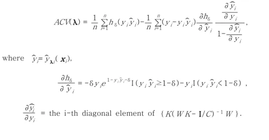
( x x x x _i ) for i = 1, ⋯, n , should be evaluated, selecting parameters using CV function is computationally formidable. By using a first order Taylor series expansion of the modified hinge loss function and the derivation procedure of GACV function from CV function by Yuan(2006), We have ACV function as follows

ACV ( λ λ λ λ) = 1 n ∑ ⁿ

i

h

( y _i ^ˆ y _i )- 1 n ∑ ⁿ

i

( y _i - y _i y ^ˆ _i ) ∂ h

∂ ^ˆ y _i

∂ ^ˆ y _i

∂ y _i 1- ∂ y ^ˆ _i

∂ y _i

, (11)

where ^ˆ y _i = ^ˆ y

_i ( x x x x _i ),

∂ h

∂ ^ˆ y _i ^{= -δ} y _i e

^y

^y

I ( y _i ^ˆ y _i ≥1-δ )- y _i I ( y _i ^ˆ y _i < 1-δ ) ,

∂ ^ˆ y _i

∂ y _i = the i-th diagonal element of { K ( W K - IIII/ C )

W } .

4. Numerical Studies 4. Numerical Studies 4. Numerical Studies 4. Numerical Studies

We illustrate the performance of SVC using IRWLS(SVC_irwls) of Section 3 by comparing with that of SVC using QP(SVC_qp) of Section 2 through the simulated example generated similar to Wahba et al.(1999).

101 data sets are generated to present the prediction performance of the proposed procedure - one for training and 100 for testing. Each data set consists of 100 x x x x ^{'s and 100} y 's. Here x x x x 's are randomly generated from (-1,1)×(-1,1).

Figure 1 shows one of 100 test data sets. The points inside the smaller circle were assigned +1. The points outside the larger circle were assigned +1. The points between circles were randomly assigned +1 with probability 0.5 and -1 with probability 0.5. In IRWLS procedure we stopped iterations when mean squared difference of two successive Lagrange multipliers is less than 0.001 The radial basis kernel function is used in this example, which is

K ( x x x x

, x x x x

)=exp(- 1

σ

|| x x x x

- x x x x

||

).

For SVC_irwls ( C ,σ

) were selected as (500, 0.7) from ACV function (11) and

δ was set to 0.0001. For SVC_qp ( C ,σ

) were selected as (500, 0.5) from CV

function (10) with replacing h

by the hinge loss function. To illustrate the

prediction performance of SVC_irwls, we compare it with SVC_qp via 100 test data sets, where the misclassification rate is used as prediction performance measure defined by

1 2 n _t ∑

n

i

(1- sign ( y ( x x x x _t

i

) ˆ( y x x x x _t

i

)) ), where x x x x _ti 's are input vectors of test data.

The averages of 100 misclassification rates from SVC_irwls and SVC_qp are obtained as 0.1252 and 0.1315, respectively. Figure 2 shows a boxplot of 100 misclassifications of both procedures. We can see that SVC_irwls has better prediction performance than SVC_qp in this example.

With simulated data sets, CPU-time of the proposed procedure are compared with that of SVC_qp computed by the built-in function of MATLAB. Table1 shows CPU-time in seconds of both procedures (run MATLAB 6.5 over Pentium IV at 2.0GHz) for SVC on a data set with different sample sizes. From table1 we can see that SVC_irwls is faster than SVC_qp.

<Figure 1> The scatter plot of 100 artificial data points ( x _t

, x _t

) of a test data

set where data point depicted by "+" represents the class1 and data

point depicted by "o" represents the class2.

<Figure 2> The boxplots of 100 misclassification rates of SVC using IRWLS and QP

<Table 1> CPU times for training SVC using IRWLS and QP

n IRWLS QP n IRWLS QP

100 0.609 1.313 300 10.375 65.875

200 2.640 16.563 400 49.968 303.500

4. Conclusions 4. Conclusions 4. Conclusions 4. Conclusions

In this paper, we dealt with obtaining the classifier by SVC_irwls and obtained ACV function for the proposed procedure. Through the example we showed that the proposed procedure derives the satisfying results. We also found that SVC using IRWLS is faster than SVC using QP which implies that the proposed procedure is appropriate for the large training data.

References References References References

1. Gunn. S. (1998). Support Vector Machines for Classification and Regression. ISIS Technical Report, U of Southhampton.

2. Kimeldorf, G. S. and Wahba, G. (1971). Some Results on Tchebycheffian Spline Functions. Journal of Mathematical Analysis and its Applications, (33), 82-95.

3. Mercer, J. (1909). Functions of Positive and Negative Type and Their

Connection with Theory of Integral Equations. Philosophical Transactions of Royal Society, A:415-446.

4. Perez-Cruz, F., Navia-Vazquez, A., Alarcon-Diana, P. L. ,and Artes-Rodriguez, A. (2000). An IRWLSprocedure for SVR. In

Proceedings of European Association for Signal Processing , EUSIPO 2000, Tampere, Finland.

5. Platt, J. (1998). Sequential Minimal Optimization: A Fast Algorithm for Training Support Vector Machines. Microsoft Research Technical Report MSR-TR-98-14.

6. Smola, A. and Scholkopf, B. (1998). On a Kernel-Based Method for Pattern Recognition, Regression, Approximation and Operator Inversion.

Algorithmica , 22, 211-231.

7. Vapnik, V. N. (1995). The Nature of Statistical Learning Theory.

Springer , New York.

8. Vapnik, V. N. (1998). Statistical Learning Theory. John Wiley , New York.

9. Wahba, G., Lin, Y. and Zhang, H. (1999). Generalized Approximate Cross Validation for Support Vector Machines, or, Another Way to Look at Margin-Like Quantities. Technical Report 1006, U. of Wisconsin.

10. Yuan, M. (2006). GACV for Quantile Smoothing Splines. Computational Statistics & Data Analysis , 50(3), 813-829.

[ received date : May. 2006, accepted date : Jul. 2006 ]