A Geometric Constraint Solver for Parametric Modeling

A Geometric Constraint Solver for Parametric Modeling

Jae Yeol Lee * and Kwangsoo Kim **

*전자통신 연구원 컴 퓨터• 소프트웨 어기 술연구소

**포항공과대학교 산업공학과

ABSTRACT

Parametric design is an important modeling paradigm in CAD/CAM applications, enabling efficient design modifications and variations. One of the major issues in parametric design is to develop a geometric constraint solver that can handle a large set of geometric configurations efficiently and robustly. In this paper, we propose a new approach to geometric constraint solving that employs a graph-based method to solve the ruler-and-compass constructible configurations and a numerical method to solve the ruler-and-compass non-constructible configurations, in a way that combines the advantages of both methods. The geometric constraint solving process consists of two phases: 1) planning phase and 2) execution phase. In the planning phase, a sequence of construction steps is generated by clustering the constrained geometric entities and reducing the constraint graph in sequence. In the execution phase, each construction step is evaluated to determine the geometric entities, using both approaches. By combining the advantages of the graph-based constructive approach with the universality of the numerical approach, the proposed approach can maximize the efficiency, robustness, and extensibility of a geometric constraint solver.

Key words : Parametric design, Variational design, Rule inferencing, Graph reduction, Geometric constraint solving

1. Introduction

Parametric design is an approach to product modeling, which associates engineering knowledge with geometry and topology in a product design by means of geometric constraints'". It allows users to make modifications to existing designs by changing parameter values. For this reason, parametric design has been considered an indispensable tool in many applications such as mechanical part design, tolerance analysis, simulations, kinematics, and knowledge-based design automation^-61.

Many research efforts have been made toward im­

proving parametric design functionality. One of the main efforts is to develop a geometric constraint solver that can solve a geometric constraint problem efficiently and robustly. There are two major ap­

proaches to solving a geometric constraint problem: 1) numerical approach and 2) constructive approach.

In the numerical approach, geometric constraints are converted into a system of numerical equations

Then, the system of equations is solved by an iterative numerical method. This approach can solve any set of geometric configurations including ruler- and-compass non-constructible configurations since any problem which can be represented as a set of equations can be, in theory, solved by numerical techniques. However, along with this advantage come some significant shortcomings1103:

-Numerical techniques have a number of problems related to numerical stability and solution consistency.

• The number of iterations required to solve a set of constraint equations can vary substantially, depending on initial conditions given to the solver.

• Numerical techniques are relatively inefficient.

• Numerical techniques cannot distinguish between different roots in the solution space.

211

212 Jae Yeol Lee and Kwangsoo Kim

Due to the limitations of the numerical approach mentioned above, most parametric design systems adopt the constructive approach as a fundamental scheme for solving geometric constraints.

In the constructive approach, geometric constraints are represented by a set of knowledge such as graphs or predicate symbols110'201. In this approach, a constraint solver satisfies the constraints by incrementally processing the set of knowledge. Usually, the solver takes two phases of geometric constraint solving: a planning phase and an execution phase. During the first phase, a sequence of construction steps is derived using a graph-based technique or a rule-based technique. During the second phase, the sequence of construction steps is carried out to determine geometric entities. The constructive approach separates the sym­

bolic aspects from the numerical aspects so that those usual problems such as numerical instabilities associated with the numerical approach can be minimized. Owen[11] presented a graph-based construc­

tive solver in which a constraint graph is analyzed for triconnected components. However, only ruler-and- compass constructible configurations were considered.

Hofftnann et aZ.[12] proposed a similar approach, but they extended their approach to deal with more complex configurations. Lee and Kim"

proposed a graph-based rule inferencing method, which can overcome an inefficient geometric reasoning process of rule-based inferencing methods. Nevertheless, it can only deal with ruler-and-compass constructible configurations.

Fig. 1 shows ruler-and-compass non-constructible models that require sophisticated solving techniques.

The triangle in Fig. 1(a) is well constrained, apart from rigid body translation and rotation. Though this configuration is seemingly very simple, it is difficult for constructive approaches to solve the constraints since it requires reasonably sophisticated ordering of construction steps. The model in Fig. 1(b) cannot be solved by any constructive approach since it partially requires a numerical technique to determine the geometric entities. These examples show that the constructive method alone cannot solve a variety of geometric configurations.

In this paper, we propose a new approach to

geometric constraint solving that employs a graph­

based method to solve the ruler-and-compass constructible configurations and a numerical method to solve the ruler-and-compass non-constructible configurations, in a way that combines the advantages of both methods. The geometric constraint solving process consists of two phases: 1) planning phase and 2) execution phase. In the planning phase, a sequence of construction steps is generated by clustering the constrained geometric entities and reducing the constraint graph in sequence. In the execution phase, each construction step is evaluated to determine the geometric entities, using both approaches. By combin­

ing the advantages of the graph-based constructive approach with the universality of the numerical approach, the proposed approach can maximize the efficiency, robustness, and extensibility of a geometric constraint solver.

The remainder of this paper is organized as follows.

Section 2 describes an overview of the proposed geometric constraint solver. Section 3 presents the construction plan generation phase of the solver.

Section 4 describes the plan evaluation phase of the solver. Section 5 shows implementations results.

Section 6 presents a conclusion with some remarks.

2. Geometric Constraint Solving: Overview

A geometric constrained problem is defined by a geometric model consisting of a set of geometric entities and a set of geometric relations, called constraints. Geometric entities used in the paper include points, lines, circles with given radii, line

한국

CAD/CAM

3

4

1998

12

segments, and circular arcs. Constraints include incidence, distance, angle, parallelism, concentricity, tangency, and perpendicularity. A geometric e

ity has its own degrees of freedom, which allow it to vary in shape, position, size, and orientation as shown in Table 1. A geometric constraint reduces the degree of freedom (DOF) of the geometric model by a certain number, called the valency of the constraint, depending on the constraint type as shown in Table

In order for a set of geometric entities to be fully constrained, all their degrees of freedom must be taken up by geometric constraints. The geometric model can be represented by a con

aint graph in which nodes are geometric entities, and edges are geometric constraints.

The proposed constraint solving process consists of two phases: 1) planning and 2) execution. In the planning phase, a sequence of construction steps is generated by incremstally forming a series of rigid bodies with three DOF (two translational, one rotational), called clusters. A rigid body is a set of geometric elements whose position and orientation relative to each other is known. At each clustering step, a rigid body with three degrees of freedom,

Table 1. Geometric entities and their degrees of freedom Geometric entities Degrees of freedom (DOF)

Point 2

Line 2

Circle 3

Cir

e with given radius 2

Table 2. Geometric constraints and their valency

Constraint Type Associated Geometric

Entities Valency

Point, Point 1

Distance Point, Line Point, Circle

1 1

Line, Line 2

Incidence Point, Line Point, Circle

1 1

Coincidence Point, Point 2

Line, Line 2

Tangency Line, Circle 1

Circle, Circle 1

Angle Line, Line 1

Parallelism Line, Line 1

Concentricity Point, Circle 2

consisting of a pair of certain geometric entities and/

or clusters and a number of geometric constraints, is identified and combined into a single merged cluster, R. This clustering process continues until the reduced constraint graph becomes a sin

e cluster.

In the execution phase, each construction step is evaluated to derive positions and orientations of the geometric entities in the cluster by selecting an appropriate solving method among the three proposed procedures described in Section 4, considering the type of clustering. If the constraint graph is not reduced to a single cluster in the planning phase, the undetermined geometric entities in the constraint graph are solved by a numerical method.

Notations being used throughout the paper are summarized below:

1) Lb G, and R represent a line, a circle, and a point, respectively.

2) Gi represents a geometric entity (or a cluster) with two DOF.

3) Ri represents a cluster (or a geometric entity) with three DOF.

3. Plan Generation

If a geometric constraint model is well-constrained as shown in Fig. 2, a sequence of construction steps, as shown in Fig. 3, is generated by two phases; 1) preprocessing the pairs of adjacent geometric entity nodes constrained by the geometric constraints with two DOF as shown in Fig. 4, and 2) clustering the pairs of adjacent geometric entity and/or cluster nodes connected by a number of constraint edges that have one of the clustering types shown in Fig. 5.

Each set of nodes/edges in Fig. 5 forms a cluster or rigid body. If a geometric model is over- or under-

한국

CAD/CAM

3

4

1998

12

214 Jae Ye

Lee and Kwangsoo Kim

(4)

(5) (3)

for the design shown in Fig. 3・ The clustering steps

Fig. 2.

constrained, a special handling of the model is neces­

sary. The preprocessing, clustering, and over- & under­

constraint detecting procedures are described below.

Li L：

Distances

* Concentric C

P Fig. 4. Constraints that reduce two degrees of freedom.

Gi： geometric entities (or clusters) with two degrees

矿

Ri： clusters (or geometric entities) with three degrees of freedom R^: geometric entities in the cluster Rt

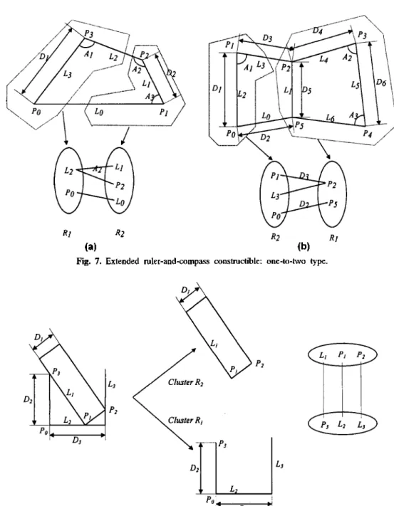
Fig. 5. Type of clustering, (a), (b): ruler-and-compass constructible, ©), (s): extended ruler-and-com- pass constructible; and (5) ruler-and-compass non-constructible configurations.

3.1 Preprocessing the constraint graph

As shown in Table 2 and Fig. 4, most of geometric constraints take up one DOF, but there are some special cases that reduce DOF by 2. A distance dimension between two lines specifies both parallelism and distance so that it takes up two degrees of freedom.

A coincidence constraint between two points also takes up two degrees of freedom, as does a concentricity constraint. These geometric constraints and their associated geometric entities are combined into a special type of clusters with 2 DOF. In the proposed approach, a cluster with 2 DOF is treated as a pseudo geometric entity with 2 DOF. During the preprocessing, thus, the set of a geometric constraint with 2 valency and its two associated geometric entities is identified and combined into a pseudo geometric entity as shown at step 0 in Fig. 3.

3.2 Clustering geometric entities and/or clusters Each set of nodes and edges shown in Fig. 5 forms a cluster or rigid body with three DOF. In this clustering procedure, the sets of nodes and edges with three DOF are identified incrementally and combined into merged nodes. By identifying and merging clusters sequentially, the constraint graph

한국

CAD/CAM

3

4

1998

12

Table 3・ Solving techniques according to clustering types

Clustering Types Type Descriptions Related Graphs

in Fig. 5

Solving Techniques

One connecting edge Two G nodes a A

Two connecting edges One G node and one R node b A

Three connecting edges One geometric entity constrained by three constraints Ci B A: Ruler-and-compass constructible (RCC)

B: Extended ruler-and-compass constructible (ERCC) C: Ruler-and-compass non-constructible (RCNC)

may be reduced to a single merged node as shown in Fig. 3. The clusters are classified into three types: 1) ruler-and-compass constructible (RCC), 2) extended ruler-and-compass constructible (ERCC), and 3) ruler- and-compass non-constructible (RCNC). An appropr­

iate solving method is provided to each of the clustering types during the execution phase as shown in Table 3.

The geometric e

ities in the clusters shown in Fig.

5(a) and 5(b) are ruler-and-compass constructible.

Thus, they can be effectively determined by a graph­

based geometric reasoning technique1171. The geometric entities in the chi

ers shown in Fig. 5(c) are not ruler-and-compass constructible. To solve this type of clusters effectively, the clusters are further classified into three types according to the relations between geometric entities in two clusters: 1) one-to- three, 2) one-to-two, and 3) one-to-one, as shown in Fig. 5©), 5(6), and 5«

respectively. One-to-three and one-to-two type clusters are solved by an extended ruler-and-compass method, whereas one-to- one type clusters are not. For example, the clusters shown in Fig. 6 & 7 are extended ruler-and-compass constructible. Note that the configurations shown in Fig.

7 cannot be solved by Aldefeld's[13] and Simde's'

rule inferencing methods because they cannot support parallelogram rules and quadrilateral rules"

The one-to-one type cluster shown in Fig. 8 is solved effectively by a numerical method. Among these clusters, however, the clusters with the con­

figuration shown in Fig. 9 can be effectively solved by a root finder for univariate polynomials1123. The difference between the two configurations in Fig. 8 and 9 lies in the constraint relation in each cluster. The configuration in Fig. 9 has a cyclic relation among geometric entities in each cluster. On the other hand, the configuration in Fig. 8 has no such a relation.

Fig. 6. Extended ruler-and-compass constructible: one- to-three type.

33 Detecting over- and under-constrained geome­

tric models

It is important to detect over- and under­

constrained conditions during constraint solving. By analyzing degrees of freedom of clusters, we can detect over- and under-constrained conditions. Let

be the total degrees of freedom of geometric entities in a cluster, and CDOF be the total degrees of freedom taken up by constraints. If GD0F<CD0F-3, then the cluster is over-constrained. If

CD0F - 3, it is under-constrained. When a cluster is marked as under-constrained, a constraint solving system may request more constraints as input, or add appropriate default constraints for an intuitive solution.

4. Plan Execution

Each construction step is evaluated to derive the positions and orientations of geometric entities in a cluster by executing an appropriate solving method described below. A ruler-and-compass constructible cluster is solved by a rule-based method". This method calculates the coordinates and coefficients of geometric entities by sele

ing appropriate rules from

한국

CAD/CAM

3

4

1998

12

216 Jae Yeol Lee and Kwangsoo Kim

(a) (b)

Fig. 7. Extended ruler-and-compass constructible: one-to-two type.

Fig. 8. Ruler-and-compass non-constructible: solvable by a numerical technique.

a rule-base and firing them. An extended ruler-and- compass constructible cluster is solved by an algebraic method. This method determines the geometric entities by finding a sequence of rotations and translations to satisfy the geometric constraints.

A ruler-and-compass non-constructible cluster is solved by a numerical method. This method solves

the constraint problem by finding a transformation matrix that represents the relation between two rigid bodies. These solving methods are explained below.

4.1 Solving the ruler-and-compass constructible clusters

In this solving procedure, the two facts are initiaDy

한국

CAD/CAM

3

4

1998

12

non-constructible: solvable by Fig. 9. Ruler-and-compass

a finder of univariate polynomials.

added into the fact-base to fix the translation and rotation of the rigid body of a geometric constraint model. For the example shown in Fig. 10, the two facts are Coordinate P； and Direction Using these facts, a rule-based inferencing process may start as shown in Fig. 11. At each step of inferencing, the rule to be fired is selected by finding a rule that is associated with the same geometric entities as those in the cunent cluster. At step 3 in Fig. 11, for instance, the selected rule is associated with two lines (£；, L» and a point (Pj) as the cluster R3. The first two conditions, Coefficient L} and Coordinate Ph in the IF-clause of the rule are satisfied by the facts added into fact-base in the previous clustering steps.

The last two conditions, On P； L3 and Angle

_{L3 Aj,} are satisfied by the two facts given by the two geometric constraints.

4.2 Solving the extended ruler-and-compass con- structible

usters

Considering the geometric entities and their relations in the chi

ers, an appropriate procedure is developed for each type of the extended ruler-and- compass constructible clusters. Each procedure

-> Coefficient L,

Coefficient

(4) >® g津

1

”

Angle L)L? A-) -> Coefficient L2

(5)

®==® —

您) 이;;

尙

Coefficient ^

丿

Coefficient -> Coordinate Pj

Fig. 11. Rule inferencing in clustering steps for the design in Fig. 10.

specifies a sequence of rotation & translation operations that transforms one cluster R} with respect to the other chi

er R2 to satisfy the geometric constraints. As an example, the procedure for the extended ruler-and-compass constructible cluster shown in Fig. 7(a) is summarized as follows. In Fig.

7(a), (i) R[ consists of L2 and Po, (ii) R2 consists of Llf P2, and

and (iii) L2 are connected to L} and P2.

PROCEDURE ONE_TO_TWO (/?；(£,P), 7?2(£,P,Z)) INPUT: two chi

ers Rj and R2

OUTPUT: a merged cluster R consisting of R} and R2 A=angle (direction(L2), direction(L；)); rotate^

£=line(P3, normal(direction(L2)));

ZP7=intersect(L, £2)； translate

vector-differ^

££=line(P0, direction(L2))；

IP2=intcrscct(LL, £0); translate^, vector-differ^

丑싱);

END_PROCEDURE

A similar procedure is given for the configuration in Fig. 7(b). In the figure, (i) Rj consists of P2 and P5,

한국

CAD/CAM

3

4

1998

12

218 Jae Ye

Lee and Kwangsoo Kim

(ii) R2 consists of L3, R, and Po, and (iii) P2 is connected to R and L3.

PROCEDURE ONE_TO_TWO(A;(P,P), R2(L,P,P)) INPUT: two clusters Rt and R2

OUTPUT: a merged cluster R consisting of Rt and R2

£=line(P2, normal(direction(£?));

ZP7=intersect(LJ) £); translate^, vector-diffe^P^ ZP));

C;=circle(P2>

7P2=intersect^J, C;); translate^, vector-differ(7P2t 3));

Z>=distance(P2, Po);

C2=circle(P2, Z>)；

G=circle(R, Z)2)J ZP3=intersect(C2, C);

A=angle (vector-differ(R-R), vector-differ(ZP3, P2));

translate^ -P2); rotate^ S); translate^ P2)；

END_PROCEDURE

4.3 Solving the ruler-and-compass non-con- structible clusters

An efficient procedure is developed to solve the ruler-and-compass non-constructible clusters. In the procedure, the constraint problem is solved by finding a transformation matrix that represents the relation between two clusters % and R2. An iterative method based on the Newton method is used to calculate a parameter, 0, for rotation and two parame­

ters for translation, dx and dy, that define a 3x3 transformation matrix. This transformation matrix is used to position the cluster R2 (or Rj) relative to the cluster Rj (or A2) so that the geometric constraints between the two clusters are satisfied.

The values of the three parameters for the trans­

formation matrix can be computed by using the iterative Newton's method given by

Xi+1 =Xl -F(X1)- (J (X，))T

where the vector X, function F(X), and Jacobian matrix J(X) are defined as follows.

~e~

X =

dy

F(X) =

f2

X)

击

히匝 d0 dd x ddy

財)

36 ddx

3

涵丑

30 dd x &&

If we position the cluster R2 relative to R}, the coordinate functions

of F(X) for the configuration shown in Fig. 8 are defined as follows.

From the constraint On P3 £;[1], f1(X)=Dx(V-P) = 0

L r.direction.x L vdirection.y

cos 6 —sin Q dx p = sin 0 cos 6 dy where D = cos 0 —sin 0

sin 0 cos 0

From the constraint On P} L2, f2(x

=Dx

y-p

= o

where

V=

L2>direction.x L2.direction,y

L 2. fointx L 2-point.y From the constraint On P2 L3,

f3(x

=Dx

y-p

= o L3.direction.x where D -

.direction.)?

Lx.foint.x L ^.pointy

1

cos 0 —sin 6 dx sin 0 cos 6 dy

⑴ A line is assumed to be defined by its direction vector and a point on the line, where direction.x is the x-coordinate value of the direction vector and point.x is the x-coordinate value of the point on the line.

한국

CAD/CAM

3

4

1998

12

and its constraint graph.

Step Clustering

(£)——쓰一(應) —*

(0): Preprocessing

丿 '

色)—으冬) —> (흐)

(1): RCC

―*■ ®

RCC —* ®

(3): RCC

①)—■* (亟)

Reduced graph

Step Clustering

RCC: ruler-and-compass constructible RCNC: ruler-and-compass non-constructible

Fig. 13. A sequence of the generated construction steps.

한국

CAD/CAM

3

4

1998

12

220 Jae Yeol Lee and Kwangsoo Kim

P =

cos 0 -sin 6 dx sin 0 cos 0 dy

i

V=

L3.foint.x L3.point.y

5. Implementation

The proposed geometric constraint solving procedures have been implemented in C++ on an IRIS Indigo2 workstation as a sub-module of the feature-based parametric modeling system developed by the authors网

Fig. 12 shows a well-constrained parametric design and its constraint graph. Though it looks to be a simple design, it is not ruler-and- compass constructible. The sequence of construction

steps generated by the proposed geometric constraint solver is shown in Fig. 13. By evaluating the sequence of construction steps for different sets of parameter values, shapes can be easily modified as shown in Fig. 14. Fig. 15 shows another example that also has a ruler-and-compass non-constructible configuration.

Each of triangles Tb T2, and T3 is ruler-and-compass constructible so that it can be solved by the rule­

based method. However, the configuration consisting of Tb T2f and T3 is ruler-and-compass non-con- structible. Fig. 16 shows a mechanical part and its modified one that are modeled by using the feature­

based parametric modeling system.

6. Discussions

We have presented a new approach to geometric constraint solving that can efficiently deal with ruler­

Fig. 15. An example design with RCNC configuration.

한국

CAD/CAM

3

4

1998

12

Fig. 16. A 3D parametric design and its modification.

and-compass non-constructible configurations as well as ruler-and-compass constructible configurations.

The proposed approach employs a graph-based constructive approach globally and a numerical approach locally. The use of the numerical approach is restricted to solving only those

usters for which it is the only approach to be applicable. By combining these two approaches, the proposed approach has the advantages of both approaches: robustness and efficiency. In this paper, we restrict the types of geometric entities to be handled to points, lines and circles. In the future, we will extend the types of geometric entities to conic sections and free-form curves such as Bezier and B-spline curves.

Acknowledgements

This research is supported in part by KOSEF(971- 1007-043-1) and ETRI.

References

1. Anderl, R. and Mendgen, R., "Parametric design and its impact on solid modeling applications", Proc.

3rd Symp. Solid Modelling Foundations & CAD/

CAM Applications, ACM Press, pp. 1-12, 1995.

2. Gossard, D.C., Zuffante, R.P. and Sakurai, H., ''Representing dimensions, tolerances, and features in MCAE systems", IEEE Comput. Graph. & Appl- ic., Vol. 5, No. 3, pp. 51-59, 1998.

3. Kondo, K

'PIGMOD: parametric and interactive geometric modeller for mechanical design", Computer- Aided Design, Vol. 22, No. 10, pp. 633-644, 1990.

4. Roller, D., "An approach to computer-aided parame­

tric design", Computer-Aided Design, Vol. 23, No.

5, pp. 385-391, 1991.

5. Solano, L. and Brunet, P., "Constructive constraint-bas­

ed model for parametric CAD systems", Computer- Aided Design, Vol. 26, No. 8, pp. 614-622, 1994.

6. Lee, J. Y., "A study on feature-based parametric design , M.S. Thesis, POSTECH, Korea, 1994.

7. Hillyard, R. and Braid, L, "Analysis of dimensions and tolerances in computer-aided mechanical design", Computer-Aided Design, Vol. 10, No. 3, pp. 161-166, 1978.

8. Kondo, K., "Algebraic method for manipulation of dimensional relationships in geometric models , Computer-Aided Design, Vol. 24, No. 3, pp. 141- 147, 1992.

9. Light, R. A. and Gossard, D. C., "Modification of geometric models through variational geometry", Computer-Aided Design, Vol. 14, No. 4, pp. 209- 214, 1982.

10. Kramer, G. A., Solving Geometric Constraint Sys- terns: A Case Study in Kinematics, MIT Press, Cam­

bridge, Massachusetts, 1992.

11. Owen, J. C., "Algebraic solution for geometry from dimensional constraints”，Proc. 1st Symp. Solid Modeling Foundations & CAD/CAM Applications, ACM Press, pp. 379-407, 1991.

12. Bouma, W., Fudos, L, Hofftnann, C. M., Cai, J. and Paige, R., "Geometric constraint solver", Computer- Aided Design, Vol. 27, No. 6, pp. 487-501, 1995.

13. Aldefeld, B., ^Variation of geometries based on a geometric reasoning method", Computer-Aided Design, Vol. 20, No. 3, pp. 117-126, 1988.

14. Sunde, G., "Specification of shape by dimensions and other geometric constraints", Geometric Model­

ing for CAD Applications, North-Holland, pp. 199- 213, 1990.

15. Suzuki, H., Ando, H. and Kimura, F., "Geometric constraints and reasoning for geometric CAD sys-

한국

CAD/CAM

3

4

1998

12

222 Jae Yeol Lee and Kwangsoo Kim

terns", Computers & Graphics, Vol. 14, No. 2, pp.

211-224, 1990.

16. Verroust, A., Schonek, F. and Roller, D., "Rule- oriented method for parameterized computer-aided design", Computer-Aided Design, Vol. 25, No. 10, pp. 531-540, 1993.

17. Lee, J. Y. and Kim, K., "Geometric reasoning for knowledge-based parametric design using graph representation", Computer-Aided Design, Vol. 28, No. 10, pp. 831-841, 1996.

18. Lee, J. Y., "A knowledge-based approach to parame­

tric feature-based modeling", Ph.D. Thesis, POS- TECH, Korea, 1998.

19. Hsu, C. and Bruederlin, A hybrid constraint solver us­

ing exact and iterative geometric constraints", CAD Systems Development: Tools and Methods, Roller and Brunet (eds.)> Springer, pp. 265-279, 1997.

**

20. Fudos, I. and Hoffmann, C. M., A graph-con­

structive approach to solving systems of geometric constraint", ACM Trans. On Graphics, Vo. 16, No.

2, pp. 179-216, 1997.

**

이 재 열

1992년 포항공과대학교 산업공학과 학사 1994년 포항공과대학교산업공학과석사 1998년 포항공과대학교 산업공학과 박사 1998년~현재 전자통신연구원但TRI) 컴 퓨터 •소프트웨어 기술연구소 동

시공학팀 시스템통합연구부 선 임연구원

관심분야 : parametric design, feature-bas­

ed modeling and geometric reasoning in intelligent CAD, Web enabled CAD, and com­

puter supported collaborative work

김 광 수

1977년 서울대학교 산업공학과 학사 1979년 서울대학교산업공학과 석사 1985년 U. of Central Florida 박사 1985년~1988년 Rochester 공과대학교

조교수

1988년 ~현재 포항공과대학교 산업공학 과 조교수/부교수

관심분야 : feature-based parametric model­

ing, feature-based NC ma­

chining, 2D & 3D geometric constraint solving, design pro­

cess automation, and virtual product modeling

한국

CAD/CAM

3

4

1998

12