- 39 -
Integer Gaussian and Reconfigurable Processor
Le Tran Su* and Jong Soo Lee*
ATRACT
Scale Invariant Feature Transform (SIFT) is an effective algorithm in object recognition, panorama stitching, and image matching, however, due to its complexity, real‐time processing is difficult to achieve with software approaches. This paper proposes using a reconfigurable hardware processor with integer half‐kernel. The integer half‐kernel Gaussian reduces the Gaussian pyramid complexity in about half [] and the reconfigurable processor carries out a parallel implementation of a full‐
search Fast‐SIFT algorithm. We use a low memory, fine grain single instruction stream multiple data stream (SIMD) pixel processor that is currently being developed.
This implementation fully exposes the available parallelism of the SIFT algorithm process and exploits the processing and I/O capabilities of the processor which results in a system that can perform real‐time image and video compression. We apply this novel implementation to images and measure the effectiveness.
Experimental simulation results indicate that the proposed implementation is capable of real‐time applications.
Key Word
SIFT, Gaussian Filter, Reconfigurable Processor, SIMD, DOG
1. Introduction
Nowadays, image matching is used to solve the many problems in computer vision, including object or scene recognition, 3D structure from multiple images, stereo correspondence, and motion tracking. In recent years,
an approach has been proposed to generate a set of salient image features. This approach has been named the Scale Invariant Feature Transform (SIFT); it transforms image data into scale‐invariant coordinates relative to local features.
The SIFT algorithm is a complex
* School of Computer Engineering & Information Technology, University of Ulsan([email protected])
#논문번호 : KIIECT2009-03-12 #접수일자 : 2009.08.24 #최종논문접수일자 : 2009.09.11
algorithm. To apply SIFT in multimedia applications, it is necessary to find a scheme to implement the algorithm in real‐time. In the SIFT algorithm, the Gaussian convolution is used in the first step to determine key
‐points. When we use a Gaussian filter mask of real coefficients; it may take a longer to obtain for calculations. To improve the performance of the SIFT algorithm a new approach has been proposed named Fast‐SIFT algorithm based on Integer Gaussian [2].
In our approach the SSE instructions are used to improve the performance of Gaussian filter calculations, with a new method to calculate the Gaussian convolution; this method is called Block Filtering. By using Block Filtering, we showed that the Gaussian filter calculations can be processed more quickly about two times than another implementation [2].
We use a parallel approach to implement the Fast‐SIFT algorithm based on Integer Gaussian. We use a single instruction stream multiple data stream pixel processor exploiting the benefits of integrating optoelectronic devices into a high performance digital processing system. By using the SIMD pixel processor system, we can expose fully the available parallelism calculation of the SIFT algorithm.
Our paper is organized as follow:
Section 2 we describe briefly the Fast
‐SIFT algorithm based on Integer Gaussian. Section 3 discusses the SIMD pixel processor system, low memory SIMD architecture. Section 4 describes in detail how the Fast‐
SIFT algorithm based on Integer Gaussian has been adapted to fully exploit the unique capability of the SIMD processor system. Strong proposals for the performance of the system and experimental results are also shown in section 4. Section 5 concludes this paper with presentation of simulation results
II. Fast Scale Invariant Feature Transform algorithm based on
integer Gaussian
The SIFT algorithm combines a scale invariant region detector and a descriptor based on the gradient distribution in the detected regions.
The descriptor is presented by a 3D histogram of gradient locations and orientations. Those descriptors (local features) are very distinctive and invariant for image scaling or rotation.
The SIFT algorithm consists of 4 main filtering stages [1]:
1. Scale‐space extreme detection:
The first stage of computation searches all scales and image locations.
2. Keypoint localization: At each candidate location, a detailed model is modelled to determine location and scale.
3. Orientation assignment: One or more orientations are assigned to each keypoint location based on local image gradient directions.
4. Keypoint descriptor: The local image gradients are measured at the selected scale in the neighbourhood of each keypoint.
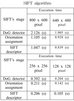
We applied the SIFT binaries provided by Lowe for various image and measured the performance. The obtained results shown that most of calculations are implemented in first state: Scale‐space extreme detection.
Therefore, to improve the performance of the SIFT algorithm implementation we concentrate to improve the performance of scale‐space extreme detection stage.
Table 1. The distribution of computation time for each stage in the
SIFT algorithm
SIFT’s stage
Execution time
800 x 600 pixel
640 x 480 pixel DoG detector 2.126 (s) 1.905 (s)
Orientation assignment
1.105 (s) 0.928 (s)
SIFT descriptor
1.047 (s) 0.839 (s)
SIFT’s stage
Execution time
256 x 256 pixel
128 x 128 pixel DoG detector 0.392 (s) 0.204 (s)
Orientation assignment
0.211 (s) 0.142 (s) SIFT
descriptor
0.206 (s) 0.105 (s)
Scale‐space extrema detection stage of the filtering attempts to equate different view points which are projections of a specific 3D object point. They are then examined in further detail. Identification of candidate locations can be efficiently achieved using the continuous "scale space" function which is based on the Gaussian function. The scale space is defined by the function:
(1)
SIFT is one such technique which locates scale‐space extrema from Gaussian image differences D(x,y,σ)
given by:
(2)
Where
* ‐ is the convolution operator, G(x, y, σ) ‐ is a variable‐scale Gaussian kernel,
I(x, y) ‐ is the input image.
k ‐ is used to up and down scale
To detect the local maxima or minima of D(x, y, σ) each point is compared with its 8 neighbours on the same scale, and its 9 neighbours on the up and down scale. If this value is larger than all 26 neighbours it is a maximum, if less a minimum.
In the Fast‐SIFT algorithm we propose a new method to implement the Gaussian convolution in scale‐
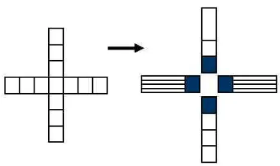
space extreme stage. In our method we use a block of 4x4 to implement the Gaussian filter. This block is shown in Figure 1.
For example we have 4x4 pixels.
This is a 4x4 block. We use a half kernel; in this case, it is an array with 4 elements. And then we put the half kernel to the block.
In figure 1 we explain the “half kernel” definition. We divide the Gaussian Kernel into 4 blocks.
Fig 1. The illustration of half kernel
These blocks will be applied to four directions (Left, Right, Top, and Bottom).
Fig 2. A 4x4 block filtering
In our new method to implement Gaussian filter, we use a 4x4 block.
This implementation includes the four steps below.
1. Load 4x4 pixels in 4 XMM registers.
2. Load 4 kernel values in a XMM register.
3. Compute convolution (Left, Right, Top, and Bottom)
Left, Right: reverse multiplication Top: Matrix transpose
Bottom: Matrix transposes then reverse multiplication
By repeating all image data we will have the output image.
III. Related works
SIFT is perhaps the most popular invariant local feature detector at present, and has been applied successfully in many occasions, such as object recognition, image match and registration, SFM & 3D reconstruction, vSLAM, image panorama, etc.
Nevertheless the complexity of the SIFT algorithm results in very high time consumption. But the high popularity of SIFT, it is no surprise that several variants and extensions of SIFT have been proposed. For example Ke and Sukthankar proposed the so called PCA‐SIFT [5] that apply Principal Components Analysis (PCA) to the normalized gradient patch. The Gradient location and orientation histogram (GLOH) [6]
changes SIFTs location grid and uses PCA to reduce the size of SIFT. The
primary focus of these extensions is to gain improved performance.
An approach named Harris – SIFT [7], by removing many indistinctive candidates before generating descriptors, Harris – SIFT saves a lot of computations. Harris – SIFT reduces both the feature number and database size, or in other words, cuts down the feature matching time. But provided results of Harris – SIFT method are not fast enough to implement in real time.
In the fast approximated SIFT [8], they proposed a modified SIFT method for recognition purpose. They speed up the SIFT computation by using approximations (mainly employing integral images) both the DoG detector (section II.1) and the SIFT descriptor (section II.4). Their method can reduce the SIFT computation time by a factor of eight compared to the binaries SIFT provided by Lowe. However, the loss in matching performance is a major drawback of this approach.
IV. SIMD Processor Array Architecture
A reconfigurable processor is a microprocessor with erasable hardware
that can rewire itself dynamically.
This allows the chip to adapt effectively to the programming tasks demanded by the particular software they are interfacing with at any given time. Ideally, the reconfigurable processor can transform itself from a video chip to a central processing unit ( CPU ) to a graphics chip, for example, all optimized to allow applications to run at the highest possible speed. In this paper we apply the SIFT algorithm in SIMD Processor.
The SIMD Pixel Processor system [4] exploits the benefits from integrating optoelectronic devices into a high performance digital processing system. In this system, an array of thin‐film detectors is integrated on top of and electrically interfaced to digital SIMD processing elements. The general architecture of a SIMD system is depicted in Figure 3. The program is stored in the array control unit (ACU), and each instruction is broadcasted to every node of the system in a lockstep fashion (i.e., via a single instruction stream). Each node, in turn, executes the received instructions on its local data (multiple data stream), while exchanging data with other nodes through the interconnection network. Each SIMD processor node is interconnected to its
four neighbours through a mesh network closed as a torus. In this way the opposite rows (or columns) of the mesh are connected to each other, enabling more powerful communication schemes than those available with a standard NEWS (North‐East‐West‐South) network.
The micro architecture of a SIMD processing element (PE) is shown in Figure 4, along with the interconnection network. The 16‐bit data path includes an adder/subtractor, barrel shifter, and multiply‐
accumulator (MACC) unit. Each PE also includes 64 words of local memory.
In addition, each SIMD processor node interfaces to a small array of thin film detectors, which is a subset of the focal plane array. The instruction set architecture allows a single node to address up to 16 x 16 arrays of detectors. Each processor incorporates eight‐bit sigma‐delta analog to digital converters to convert light intensities, incident on the detectors, into digital values. The SAMPLE instruction simultaneously samples all detectors values and makes them available for further processing. The SIMD execution model allows the entire image projected on many nodes to be sampled in a single cycle.
This monolithic integration is the key – feature of the SIMD Pixel Processor system, providing an extremely compact, high frame rate, focal – plane processing.
P0
MEM 0 P1
MEM 1
Pn
MEM n P0
MEM 0 P1
MEM 1
Pn
MEM n
ACU
INTERCONNECTION NETWORK INSTRUCTION STREAM
Fig 1. Organization of a SIMD parallel architecture
Neighboring PEs
Comm. Unit
Register File 16 by 32 bit 2 read, 1 write
CFA S&H and ADC
SP.Registers&I/O
Arithmetic, Logical, and Shift
Unit
MACC
MMX
Local memory
Sleep Decoder
Single Processing Element
Fig 2. A block diagram of a SIMD processor array
V. Implement Fast‐SIFT in SIMD parallel architecture
To carry out the Fast‐SIFT algorithm, we consider all pixels of the images. By using the specified SIMD array, we distribute all pixels
into all PEs in which every PE owns 16 pixels. Assume n is the total number of pixels. As a result, the number of PEs involved in the computation is n/16. By dividing the pixels among n/16 processors, every PE caries out the computation only on the local memory containing 16 owned pixels along with their membership values as well as center values. Then, the Fast‐SIFT algorithm is implemented on n/16 processors in which some new equations are required for every PE. This enhances the performance of Fast‐SIFT algorithm implementation.
The first stage of Fast‐SiFT algorithm includes two steps: DOG (difference of Gaussian) space construction and extrema detection.
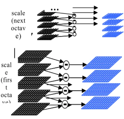
Figure 5 shows the process of building DOG space. The input image will be resized to build scale space. In each scale space, we apply new approach to implement Gaussian filter for images. After subtraction of blurred images we get DOG space.
Figure 6 describes DOG space and how to detect the extrema. To detect the local maxima or minima, each point is compared with its 8 neighbours on the same scale, and its 9 neighbours on the up and down scale. If this value is larger than all
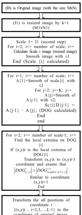
26 neighbours it is a maxima, if less a minima. Figure 7 shows the flowchart of keypoints detection.
Fig 5. DoG space construction
SIMD processor architecture provides a suitable way to implement the DOG space construction. Two levels of parallelism are exploited in this implementation. One is image scaling process. Second is applying Gaussian filter. We will describe in more detail these steps in the next section.
Fig 6. DoG space scale
1. Image scaling
The purpose of this step is constructing scale space. The original image will be resized by a constant k.
In my implementation k = 0.5.
The image scaling process is described in Figure 6. In this step, first we shrink the image to the left.
Each pair of adjacent pixels will be replaced by a new one. The value of new pixel is the mean value of these pixels. After shrinking the image to the left, we implement shrinking image to the bottom. In this way, we get the resized image.
…
scal e (firs
t octa
ve) scale (next octav
e)
(I0) is Original image (with the size MxN)
(I1) is resized image by k>1 (M1xN1)
Scale 1= I1 (second step) For i=2; i<= number of scale; i++
Calculate Scale i image (resized image) Smooth image with s1
End (Scale {i} calculated)
For i=1; i<= number of scale; i++
A{1}=Smooth of scale{i} with s2
For j=2; j<=K; j++
A{j}=Smooth of A{j‐1} with s2;
Sc{i}D{j‐1} = A{j‐1} ‐ A{j}; (DOG calculated)
End end
For i=2; i<= number of scale‐1; i++
Find the local extrema on DOG {i}
If (x,y)i is the local extrema of DOG{i}
Transform (x,y)i to (x,y)i‐1 coordinate and ensure that
( ) ( )
1 , ,
> neighbori+ of xy i
y
x DOG
DOG
Similar to coordinate (x,y)i+1
End
Transform the all positions of coordinate i
{(x,y)i , i=2,3,…,L‐1} to the coordinate of original image.
Fig 7. Flowchart of keypoint detection algorithm
Left
Bottom
Figure 8: Image scaling process
(a) (b) (c)
Fig 9. Scale space images (a) 1st octave (b)2nd octave (c)3rd octave
2. Gaussian filter
As we described in section II, in our method we use a block filtering technique to implement Gaussian filter.
Original image Blurred image Fig 10. Difference of Gaussian image
VI. Performance Evaluation
To evaluate the performance of the proposed algorithm, we use a cycle accurate SIMD simulator. We developed the parallel Fast‐SIFT algorithm in their respective assembly languages for the SIMD processor array. In this study, the image size of 256 × 256 pixels is used. For a fixed 256 × 256 pixel system, because each PE contains 4x4 pixels so the number of 4,096 PEs is used.
We summarize the parameters of the system configuration in table 2.
The metrics of execution time and sustained throughput of each case form the basis of the study comparison, defined in (8) and (9)
Execution time
(8) Sustained throughput
(9)
Where C is the cycle count, fk is the clock frequency, Oexec is the number of executed operations, U is the system utilization, and NPE is the number of processing elements.
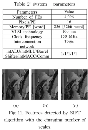
Table 2. system parameters Parameters Value Number of PEs 4,096
Pixels/PE 16
Memory/PE [word] 256 [32bit word]
VLSI technology 100 nm Clock frequency 150 MHz
Interconnection network
Torus intALU/intMLU/Barrel
Shifter/intMACC/Comm 1/1/1/1/1
(a) (b) (c)
Fig 11. Features detected by SIFT algorithm with the changing number of
scales.
Figure (11.a): number of octave is 2, (11.b) and (11.c) are 3 and 4 respectively.
Figure 11 presents the detected SIFT features with Lena image. As the number of scale is higher the detected SIFT features is more exactly.
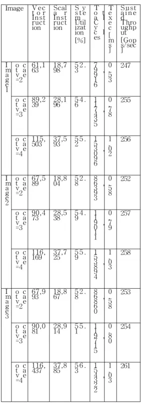
Table 3 summarizes the execution parameters for each image in the 4,096 PE system. Scalar instructions control the processor array. Vector instructions, performed on the processor array, execute the algorithm in parallel.
System Utilization is calculated as the average number of active processing elements. The algorithm operates with
System Utilization of 54% in average, resulting in high sustained throughput.
Overall, our parallel implementation supports sufficient performance of real time (30 frame/sec or 33 ms) and provides efficient processing for the SIFT algorithm.
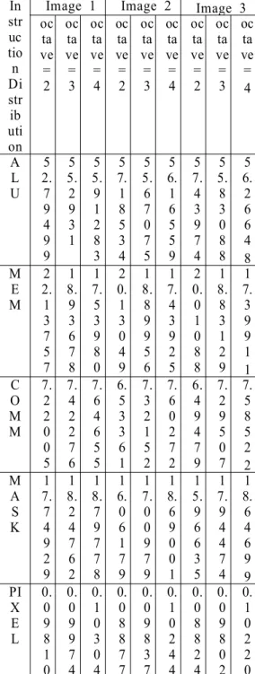
Table 4 shows the distribution of vector instructions for the parallel algorithm. Each bar divides the instructions into the arithmetic‐logic
‐unit (ALU), memory (MEM), communication (COMM), PE activity control unit (MASK), and image loading (PIXEL). The ALU and MEM instructions are computation cycles while COMM and MASK instructions are necessary for data distribution and synchronization of the SIMD processor array. Results indicate that the proposed algorithm is dominated by ALU, MEM and MASK operations.
Table 5 shows the comparison between our parallel implementation with the SIFT binaries implementation and the SIFT implementation based on OpenCV . The results indicate that our method can reduce the performance by around 390 times to SIFT binaries method and 230 times to OpenCV‐
based implementation. These results demonstrate that the proposed parallel approach supports fast performance and also provide reliable and efficient processing for SIFT implementation
Table 3. Algorithm performance on a 4,096 PE system running at 150MHz.
Image Ve ct o r Instruct ion
Scala r Instruct ion
S ys t e mUtil ization [%]
To t a lC yc l es
Te xe c[ ms ]
Susta i n e dThro ughput [Gops/sec ] Im
ag e1
o ct a v e=2
61,163 18,7 98 5 2 .
3 7
9 ,9 16
0. 53
247
o ct a v e=3
89,239 28,1 96 5 4 .
6 1
17 , 43 5
0. 78
255
o ct a v e=4
115,503 37,5 93 5 5 .
2 1
53 , 09 6
1. 02
256
Im ag e2
o ct a v e=2
67,589 18,8 04 5 2 .
8 8
6 ,3 93
0. 58
252
o ct a v e=3
90,473 28,5 38 5 4 .
9 11 9 ,0 11
0. 79
257
o ct a v e=4
116,169 37,7 25 5 5 .
9 1
53 , 89 4
1. 03
258
Im ag e3
o ct a v e=2
67,993 18,8 67 5 2 .
8 86 , 86 0
0. 58
253
o ct a v e=3
90,081 28,9 14 5 5 .
1 1
19 , 71 5
0. 80
254
o ct a v e=4
116,437 37,8 85 5 6 .
3 15 4 ,3 22
1. 03
261
Table 4. The distribution of vector instructions for the algorithm In
str uc tio n Di str ib uti on
Image 1 Image 2 Image 3 oc
ta ve
= 2
oc ta ve
= 3
oc ta ve
= 4
oc ta ve
= 2
oc ta ve
= 3
oc ta ve
= 4
oc ta ve
= 2
oc ta ve
= 3
oc ta ve
= 4
A L U
5 2.
7 9 4 9 9
5 5.
2 9 3 1
5 5.
9 1 2 8 3
5 7.
1 8 5 3 4
5 5.
6 7 0 7 5
5 6.
1 6 5 5 9
5 7.
4 3 9 7 4
5 5.
8 3 0 8 8
5 6.
2 6 6 4 8 M
E M
2 2.
1 3 7 5 7
1 8.
9 3 6 7 8
1 7.
5 3 9 8 0
2 0.
1 3 0 4 9
1 8.
8 9 9 5 6
1 7.
4 3 9 2 5
2 0.
0 1 0 8 8
1 8.
8 3 1 2 9
1 7.
3 9 9 1 1 C
O M M
7.
2 2 0 0 5
7.
4 2 2 7 6
7.
6 4 6 5 5
6.
5 3 3 6 1
7.
3 2 1 5 2
7.
6 0 2 7 2
6.
4 9 4 7 9
7.
2 9 5 0 7
7.
5 8 5 2 2 M
A S K
1 7.
7 4 9 2 9
1 8.
2 4 7 6 2
1 8.
7 9 7 7 8
1 6.
0 6 1 7 9
1 7.
0 0 9 7 9
1 8.
6 9 0 0 1
1 5.
9 6 6 3 5
1 7.
9 4 4 7 4
1 8.
6 4 6 9 9 PI
X E L
0.
0 9 8 1 0
0.
0 9 9 7 4
0.
1 0 3 0 4
0.
0 8 8 7 7
0.
0 9 8 3 7
0.
1 0 2 4 4
0.
0 8 8 2 4
0.
0 9 8 0 2
0.
1 0 2 2 0
Table 5: Compare the performance with the implementation of original SIFT
Image Time execution
SIFT binari
es [ms]
OpenC V Imple mentati
on [ms]
Our metho
d [ms]
Ima ge 1
Oct ave
= 2
343 217 0.53
Oct ave
= 3
367 227 0.78
Oct ave
= 4
393 234 1.02
Ima ge 2
Oct ave
= 2
350 220 0.58
Oct ave
= 3
378 231 0.79
Oct ave
= 4
401 245 1.03
Ima ge 3
Oct ave
= 2
351 225 0.58
Oct ave
= 3
379 239 0.80
Oct ave
= 4
394 251 1.03
VII. Conclusion
In this paper, a parallel implementation of the Fast‐SIFT algorithm based on Integer Gaussian on a SIMD pixel processor has been presented. By using the SIMD pixel processor system, we exposed fully the available parallelism of the Fast‐
SIFT algorithm especially in the DoG space construction step. Preliminary simulation results suggest that the SIMD processor system can deliver real‐time performance for the Fast‐
SIFT algorithm.
Acknowledgements
This research was supported by the ADD (Agency for Defense Development) project developing an autonomous vehicle using multiple sensors.
Reference
[1] D. Lowe, “Distinctive Image Features from Scale‐Invariant Keypoints,” IJCV 60(2):91‐110, 2004
[2] Le Tran Su, Phil Jung Ghang and Jong soo Lee, “Integer Gaussian
Convolution with cache memory for real – time processing of the Scale Invariant Feature Transform Algorithm”, ITC‐CSCC 2007, Busan, Korea, 2007
[3] Lowe, D. G., “Object recognition from local scale‐invariant features”, International Conference on Computer Vision, Corfu, Greece, September 1999
[4] D. Lowe, “Distinctive Image Features from Scale‐Invariant Keypoints,” IJCV 60(2):91‐110, 2004
[5] The Pica Group, “the SIMD Pixel Processor: Micro‐architecture, Instruction Set and Programmer’s Model”, Fine‐Grain Parallel System Laboratory, School of ECE, Georgia Institute of Technology, 1995.
[6] Ke, Y., Sukthankar, R.: PCA‐
SIFT: A more distinctive representation for local image descriptors. In: Proc. CVPR.
Volume 2. (2004) 506–513
[7] Mikolajczyk, K., Schmid, C.: A performance evaluation of local descriptors. IEEE Trans. PAMI 27 (2005) 1615–1630
Ning Xu, Wei‐dong Chen , A High Real‐time and Robust Object Recognition and Localization Algorithm, China Journal of Image and Graphics, October 2007
[8] M. Grabner, H. Grabner, and H.
Bischof. Fast approximated sift. In P.J. Narayanan, editor, Proc. 7th Asian Conference on Computer Vision, volume LNCS 3851, pages 918–927. Springer, 2006
저자약력
Full name: Le Tran Su Born: 1982
Student of High Quality Engineer Training Progr am
(Program with co-opera tion of French Embass y) in Hanoi University of Technology. Gra duated with “Excellent Engineer” degree.
Major in Information and Communication S ystem
Got Master degree in University of Ulsan Now is Phd Candidate at Multimedia Appl ication Laboratory, University of Ulsan
Jong Soo Lee received his Bachelors degree in Electrical Engineering in 1973 from Seoul National University and his M.Eng.
in 1981 and Ph.D degree in 1985 from Virginia Polytechnic Institute and State University in the USA. He is currently working in the area of multimedia at the University of Ulsan in Korea. His research interests include development of personal English cultural experience programs using multimedia and 3D user interface techniques to facilitate the acquisition of English language skills by Koreans.