Simulation study on the estimation of multinomial proportions

Simulation study on the estimation of multinomial proportions

Daehak Kim ¹

1 Department of Mathematics, Catholic University of Daegu

Received 29 February 2012, revised 20 March 2012, accepted 23 March 2012

Abstract

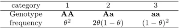
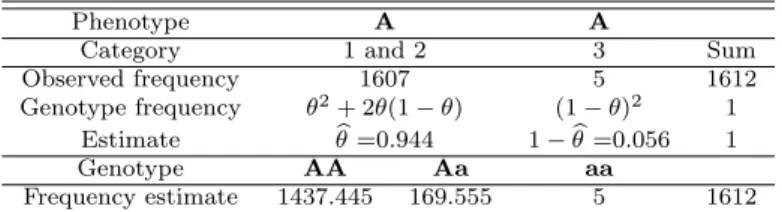
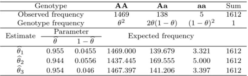
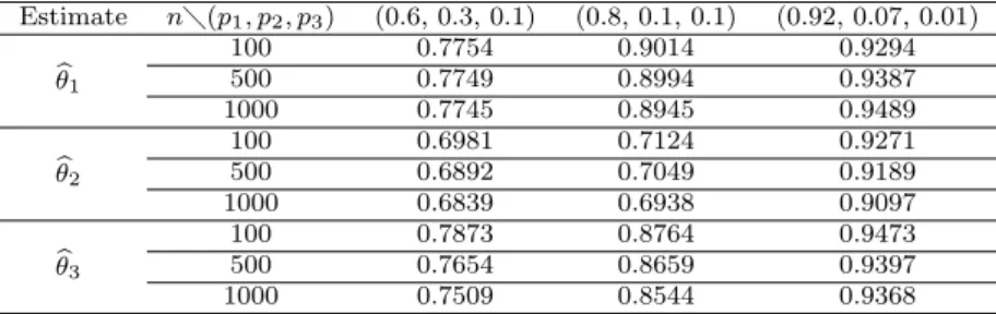
In this paper, we consider the estimation of multinomial proportions. Multinomial distribution is the most important multivaritate distribution. Estimation of multino- mial parameters for multinomial distribution is widely applicable to many practical research areas including genetics. We investigated the properties of several frequency substitution estimates and derived the maximum likelihood estimate of multinomial proportions of Hardy Weinberg proportions. Phenotype and genotype frequencies of allele are used to the estimation of multinomial proportions. These estimates are then analyzed via numerical data. Small sample Monte Carlo simulation is conducted to compare considered estimates of multinomial proportions.

Keywords: Hardy Weinberg proportions, Monte Carlo simulation, multinomial distri- bution, phenotype allele, proportion estimation.

1. Introduction

The multinomial distribution is the most important multivariate distribution on discrete data. The multinomial distribution applies when we have a random experiment with n possible results, which belong to mutually exclusive categories with unknown probabilities.

Once we have constructed a statistical model, we usually want to estimate parameters of the unknown distribution generating the data. If the model is given by the family of the distributions of random variable, then any quantity we are trying to estimate can be thought of as a real-valued function of q on the parameter space. For instance, in the hyper- geometric distribution, the number of defectives in the shipment can be thought of as the function q(θ), where θ is the fraction of defectives. To estimate q(θ) we select a statistic T and evaluate it at the outcomes of the experiment. Thus if the true value of θ is θ 0 , we observe samples and are using the estimate T , our guess at the unknown number q(θ ₀ ) is the known number T . How do we select reasonable estimates for a given function q(θ)?

For the multinomial proportions and the estimation of statistical parameters, there are abundant results. Pearson (1903) had studied a mathematical contributions to the theory of evolution in the sense of the influence of natural selection on the variability and correlation of organs. Lee and Lee (2012) had studied an approximate maximum likelihood estimation

1

Professor, Department of Mathematics, Catholic University of Daegu, Kyungsan 712-702, Korea.

E-mail: [email protected]

in a weighted exponential distribution. Cho (2006) also considered multiple comparison of the proportions for negative binomial populations using fractional bayes factor. Kang (2003) had studied the bootstrap method for the estimation of negative binomial parameter. Lee et al. (2006) conducted a simulation study on gene-environment interaction. On the while, Park (2011) had studied the estimation of error variance and Park and Km (2011) considered the estimation of the treatment effect for censored data. Shi et al. (2011) had studied the genetic diversity and distances using microsatellite markers.

In this paper, we introduce two methods of estimation, frequency substitution principle and maximum likelihood respectively for the multinomial distribution. Particularly, we de- rive maximum likelihood estimator of Hardy Weinberg proportions. Then, these two meth- ods of estimation are applied to the Hardy Weinberg proportions. In this case, we consider two ways of estimation of proportions. One is based on genotype frequency and the other is based on phenotype frequency. Also, Monte Carlo simulation is conducted to compare the performance of estimates.

The rest of this paper is organized as follows. In section 2, simple view of estimation methods for the multinomial parameters is given. In section 3, we estimate the Hardy Weinberg proportions based on genotype frequency and phenotype frequency respectively via numerical example. Simulation is conducted in section 4 in order to compare the considered estimates. Conclusion is given in section 5.

2. Estimation methods for multinomial proportions

2.1. Frequency substitution estimate

Suppose we observe n multinomial trials for k categories but their respective probabilities p 1 , p 2 , · · · , p k are completely unknown. If we let N i be the number of items belong to the ith category, i = 1, 2, · · · , k, then the simplest intuitive estimate of p i is N i /n, the proportions of sample values belong to ith category. As an illustration, consider a population of men whose occupations fall in one of five different status categories, 1, 2, 3, 4 or 5. Table 2.1 shows some job category data. Here, k = 5, p _i is the proportions of men in the population in the ith job category, and N _i /n is the sample proportions in this category. Mosteller (1968) used the data of Table 2.1 for the association and estimation in contingency tables.

Table 2.1 Job category data

i 1 2 3 4 5 sum

N

23 84 289 217 95 n =708

p b

0.03 0.12 0.41 0.31 0.13 1

Next, consider the more general problem of estimating a continuous function q(p 1 , · · · , p k ) of the population proportions. The most natural approach is given by the frequency substi- tution principle whereby we replace the unknown population frequencies p 1 , p 2 , · · · , p k by the observable sample frequencies N 1 /n, · · · , N k /n. That is, use

T = q N 1

n , · · · , N k

n

!

to estimate q(p ₁ , · · · , p _k ). For instance, suppose that in the previous job category data in Table 1, categories 4 and 5 correspond to blue collar jobs, while categories 2 and 3 correspond to white collar jobs. We would be interested in estimating

q(p 1 , · · · , p 5 ) = (p 1 + p 3 ) − (p 2 + p)

the difference in the proportions of blue collar and white collar workers. If we use the frequency substitution principle, the estimate is

T = N 1

n + N 3

n

!

− N 2

n + N 4

n

!

which in our case is 0.44 − 0.43. For details, see Bickel and Doksum (1977).

2.2. Hardy Weinberg proportions

Now suppose that the proportions p 1 , p 2 , · · · , p k do not vary freely, but are continuous functions of some m dimensional parameter θ = (θ 1 , · · · , θ m ) and that we want to estimate a component of θ or more generally a function q(θ). Many of the models arising in the analysis of discrete data are of this type. A simple example is given by sampling from a population in genetic equilibrium with respect to a single gene with two allele. If we assume the three different genotype are identifiable, we are led to suppose that there are three types of individuals whose frequencies are given by the so-called Hardy Weinberg proportions (or Hardy Weinberg principles, Hardy Weinberg equilibrium)

p ₁ = θ ² , p ₂ = 2θ(1 − θ), p ₃ = (1 − θ) ² (2.1) where 0 < θ < 1. For details about Hardy Weinberg proportions, see Stern (1943).

The Hardy Weinberg principle states that both allele and genotype frequencies in a pop- ulation remain constant, that is, they are in equilibrium from generation to generation un- less specific disturbing influences are introduced. Those disturbing influences include non- random mating, mutations, selection, limited population size, “overlapping generations”, random genetic drift, gene flow and meiotic drive. It is important to understand that out- side the lab, one or more of these “disturbing influences” are always in effect. That is, Hardy-Weinberg equilibrium is impossible in nature. Genetic equilibrium is an ideal state that provides a baseline against which to measure change.

Static allele frequencies in a population across generations assume no mutation (the al- lele don’t change), no migration or emigration (no exchange of allele between populations), infinitely large population size, and no selective pressure for or against any genotype. Geno- type frequencies will also be static when mating is random.

In the simplest case of a single locus with two allele, the dominant allele is denoted A and the recessive a. Their frequencies are denoted by θ and 1 − θ respectively, so θ + (1 − θ) = 1.

The final three possible genotype frequencies in the offspring become as in Table 2.2.

If N _i is the number of individuals of ith category in the sample of size n, then (N ₁ , N ₂ , N ₃ ) has a multinomial distribution with parameters (n, p ₁ , p ₂ , p ₃ ) given by (2.1). Suppose we want to estimate θ, the frequency of one of the allele. Since θ = √

p 1 , we can use the

substitution principle and estimate by pN 1 /n. Note however, that we can also write θ =

Table 2.2 Hardy Weinberg equilibrium

category 1 2 3

Genotype AA Aa aa

frequency θ

2θ(1 − θ) (1 − θ)

1 − √

p ₃ and thus 1 − pN ₃ /n is also plausible estimate of θ. In general, suppose that we want to estimate a continuous function q of θ. If p ₁ , p ₂ , · · · , p _k are continuous functions of θ, we can usually express q(θ) as a continuous function of p ₁ , p ₂ , · · · , p _k .

2.3. Maximum likelihood estimation

The method of maximum likelihood was first proposed by the German mathematician Gauss. However the approach is usually credited to the English statistician Fisher (1922) who rediscovered the idea in his paper. The method of maximum likelihood consists of finding that value b θ of the parameter which is most likely to have produced the data. That is, for given data, we seek b θ which satisfies

L(b θ) = max L(θ), θ ∈ Θ.

If such a b θ exists, we estimate any function q(θ) by q(b θ). The estimate q(b θ) is called the maximum likelihood estimate of q(θ).

Let (N 1 , N 2 , N 3 ) be a random sample from a multinomial distribution with parameters (n, p 1 , p 2 , p 3 ) occurring in the Hardy Weinberg proportions. That means N i is the number of individuals of ith category in the sample of size n. The likelihood function can be written as

L(θ) = (θ ² ) ^N

2θ(1 − θ) ^N2 (1 − θ) ^N

= 2 ^N

θ ^2N

^+N

(1 − θ) ^N

^+2N

and log likelihood

logL(θ) = 2(N 1 + N 2 ) log θ + (N 2 + 2N 3 ) log(1 − θ).

So it may be easier to solve the following equation

∂

∂θ logL(θ) = 2N 1 + N 2

θ − N 2 + 2N 3

1 − θ = 0. (2.2)

By solving equation (2.2), we can get the maximum likelihood estimator of Hardy Weinberg proportions θ by

θ = b 2N ₁ + N ₂

2n . (2.3)

3. Estimation of Hardy Weinberg proportions

Unfortunately, violations of assumptions in the Hardy Weinberg principle does not mean

the population will violate Hardy Weinberg equilibrium. For example, balancing selection

leads to an equilibrium population with Hardy Weinberg proportions. This property with selection versus mutation is the basis for many estimates of mutation rate (call mutation- selection balance).

3.1. Proportion estimation based on phenotype frequency

Suppose that the phenotype of AA and Aa are indistinguishable, that is, there is complete dominance. Assuming that Hardy Weinberg principle applies to the population, then the proportions of recessive a can be calculated from the equation

(1 − θ) ² = N ₃ /n.

By solving this equation, we can get the estimate b θ θ = 1 − b p

N 3 /n (3.1)

as proportions of dominance A. These are summarized in Table 3.1. For example, we used the data in Table 3.1 from Ford (1971) on the Scarlet tiger moth, for which the phenotype of a sample of the populations were recorded.

Table 3.1 Estimation based on phenotype

Phenotype A A

Category 1 and 2 3 Sum

Observed frequency 1607 5 1612

Genotype frequency θ

+ 2θ(1 − θ) (1 − θ)

1

Estimate θ =0.944 b 1 − b θ =0.056 1

Genotype AA Aa aa

Frequency estimate 1437.445 169.555 5 1612

In this case, we can get only one possible substitution estimate. It is notable that there is no possible maximum likelihood estimator like (2.3).

3.2. Proportion estimation based on genotype estimation

Now, consider the same previous data on the Scarlet tiger moth but assume we know the genotype exactly.

In this case, we can get several estimates of population frequency of dominant allele A as explained in section 2.2 and 2.3. Table 3.2 shows the structure of genotype frequency and genotype.

Table 3.2 Genotype and frequency

Category 1 2 3 Sum

Genotype AA Aa aa

Observed frequency 1469 138 5 1612

Genotype frequency θ

2θ(1 − θ) (1 − θ)

1

Let the first frequency substitution estimator be b θ 1 and the second frequency substitution

estimator b θ 2 , respectively. And let us denote maximum likelihood estimator by b θ 3 . So we

can get these three estimates as

θ b 1 = p

N 1 /n, b θ 2 = 1 − p

N 3 /n, b θ 3 = 2N 1 + N 2

2n .

By using these estimates, we can get the Hardy Weinberg proportions estimates respec- tively. The results are showed in the Table 3.3.

Table 3.3 Estimation based on genotype frequency

Genotype AA Aa aa Sum

Observed frequency 1469 138 5 1612

Genotype frequency θ

2θ(1 − θ) (1 − θ)

1 Estimate Parameter

Expected frequency θ b 1 − b θ

θ b

0.955 0.0455 1469.000 139.679 3.321 1612 θ b

0.944 0.0556 1437.445 169.555 5.000 1612 θ b

0.954 0.046 1467.397 141.206 3.397 1612

In this case, the second frequency substitution estimator b θ 2 has the same value as the result of based on phenotype frequency appeared in previous section. Of course, the expected frequency of each genotype can be used for appropriate significance test. In this case, null hypothesis is that the population is in Hardy Weinberg proportions and the alternative hypothesis is that the population is not in Hardy Weinberg proportions. It can provide an interesting statistical results.

4. Simulation.

In order to compare the performance of three estimators b θ 1 , b θ 2 and b θ 3 mentioned at section 3.2, we considered small sample Monte Carlo simulation. For the simulation, we used IMSL subroutines for Fortran program. It provides the multinomial random number generation routines named RNMTN.

We considered three categories only in multinomial distribution in ordet to get the Hardy Weinberg proportions estimation. For the parameters (n, p 1 , p 2 , p 3 ) of multinomial distribu- tion, we considered the following structure in Table 4.1. For simulation, we can only consider the proportions estimation based on genotype frequency due to the limitation of phenotype frequency.

Table 4.1 Simulation design

Category 1 2 3 trials

Genotype AA Aa aa n

Genotype frequency p

= θ

p

= 2θ(1 − θ) p

= (1 − θ)

Multinomial trials n are chosen as 100, 500, 1000, respectively. For each trials, we used the genotype frequency (p 1 , p 2 , p 3 ) as (0.6, 0.3, 0.1), (0.8, 0.1, 0.1) and (0.9, 0.07, 0.01) respectively. All simulation was conducted in personal computer based on 1000 replications.

Simulation results are shown in Table 4.2.

From the Table 4.2, we can find that estimated average values are not so much vary as

trial n increases but vary so much as parameter (p ₁ , p ₂ , p ₃ ) change.

Table 4.2 Estimated average values of proportions b θ of dominance allele A Estimate n(p

, p

, p

) (0.6, 0.3, 0.1) (0.8, 0.1, 0.1) (0.92, 0.07, 0.01)

θ b

100 0.7754 0.9014 0.9294

500 0.7749 0.8994 0.9387

1000 0.7745 0.8945 0.9489

θ b

100 0.6981 0.7124 0.9271

500 0.6892 0.7049 0.9189

1000 0.6839 0.6938 0.9097

θ b

100 0.7873 0.8764 0.9473

500 0.7654 0.8659 0.9397

1000 0.7509 0.8544 0.9368

5. Conclusion and remarks

We considered the estimation of multinomial proportions, particularly, Hardy Weinberg proportions. Maximum likelihood estimation and frequency substitution estimation were considered for the estimation of Hardy Weinberg proportions based on phenotype frequency and genotype frequency respectively. From the numerical study and simulation, we can know frequency substitution estimator b θ 2 can be used to the estimation of proportions based phenotype frequency and maximum likelihood estimator b θ 3 can be used to the proportions estimation based on genotype frequency.

In real world, estimation of proportions of dominance A based on phenotype frequency is more general. For practical applications, not only maximum likelihood estimation but also frequency substitution estimation can be useful tool.

References

Bickel, P. J. and Doksum, K. A. (1977). Mathematical statistics: Basic ideas and selected topics, Holden- Day, Inc.

Cho, J. S. (2006). Multiple comparison of the proportions for negative binomial populations using fractional Bayes factor. Journal of the Korean Data Analysis Society, 8, 1361-1368.

Fisher, R. A. (1922). On the mathematical foundations of theoretical statistics, reprinted in contributions to mathematical statistics, John Wiley & Sons, New York.

Ford, E. B. (1971). Ecological genetics, Chapman and Hall, London.

Kang, C. (2003). Bootstrap method for the estimation of negative binomial parameter k. Journal of the Korean Data Analysis Society, 5, 519-525.

Lee, J. C. and Lee, C. S. (2012). An approximate maximum likelihood estimator in a weighted exponential distribution. Journal of the Korean Data & Information Science Society, 23, 219-225.

Lee, J. W., Kim, H. Lee, H. J. (2006). A simulation study on gene-environment interaction. Journal of the Korean Data Analysis Society, 8, 927-938.

Mosteller, F. (1968). Association and estimation in contingency tables. Journal of the American Statistical Association, 63, 1-28.

Park, C. G. (2011). Estimation of error variance in nonparametric regression under a finite sample using ridge regression. Journal of the Korean Data & Information Science Society, 22, 1223-1232.

Park, H. I. and Kim, J. S. (2011). An estimation of the treatment effect for the right censored data. Journal of the Korean Data & Information Science Society, 22, 537-547.

Pearson, K. (1903). Mathematical contributions to the theory of evolution, XI. On the influence of natural selection on the variability and correlation of organs. Philosophical Transactions of the Royal Society of London A, 1-66.

Shi, Z., Lee, J. H, Lee, Y. S., Oh, D. Y. and Yeo, J. S. (2011). Analysis of genetic diversity and distances in Asian cattle breeds using microsatellite markers. Journal of the Korean Data & Information Science Society, 21, 795-802.

Stern, C. (1943). The Hardy-Weinberg law. Science, 97, 137-138.