† 정회원, 고려대학교, 건축·사회 환경공학과, 교수 E-mail : [email protected]
TEL : (02)3290-3317 FAX : (02)921-5166
* 비회원, 고려대학교, 건축·사회 환경공학과, 박사과정
** 정회원, 고려대학교, 건축·사회 환경공학과, 박사과정
*** 정회원, 한국철도기술연구원, 차륜궤도연구실, 선임연구원
헤르쯔 접촉스프링과 레일 요철을 고려한 차량-교량 동적상호작용 비선형 해석
Nonlinear Dynamic Analysis of Vehicle-Bridge Interaction considering the Hertzian Contact Spring and Rail Irregularities
강 영 종† 웬 판 반* 김 정 훈** 강 윤 석***
Young-Jong Kang Van-Ban Nguyen Jung-Hun Kim Yoon-Suk Kang
ABSTRACT
In this paper, the nonlinear dynamic response of Vehicle-Bridge interaction with the coupled equations of motion including nonlinear Hertzian contact is presented. The moving train model is chosen to have 10 degrees of freedom (DOF). The bridge is modeled as 2D Euler-Bernoulli beam element with 4 DOF for each element, two for rotations and another two for translations. The nonlinear Hertzian contact is used to simulate the interaction between vehicle and bridge. Base on the relationship of wheel displacement of the vehicle and the vertical displacement of the bridge in Hertzian contact, the coupled equations of motion of the whole system is derived. The convenient formulation was encoded into a computer program. The contact forces, contact area and stress of the rail surface were also computed. The accuracy and efficiency of the proposed program are verified and compared with exact analytical solution and other previous studies. Various numerical examples and parametric studies have demonstrated the versatility and applicability of the proposed program.
1. Introduction
Since very first railway system was operated, the “ratting during the motion” has been observed and studied. Although nowadays, the problem may have been reduced, the problems of rail – vehicle dynamics resulting from the moving contact points between wheels and rails are as much concern today as they were over 150 years ago [1]. Generally, only the bridge response is concerned, and vehicle is just simply modeled as moving load. However, when the weight of the vehicle increase, such as for the case of railway train. The inertial and the dynamic forces are needed to taken into account. The moving load model also cannot concerning the vehicle response. There are many researchers interested in this problem. In [2] only vehicle is investigated while in [3] only track system is concerned. In this study, the vehicle and bridge will be model as one system, and the convenient coupled equations of motion are encoded into a computer program. The proposed program is verified with exact analytical results, the good agreements are obtained. As a result, the proposed program is applied to analysis the responses of a real vehicle model of Korea eXpress Train (KTX)
2. Equations of Motion
2.1 Bridge Equations of Motion
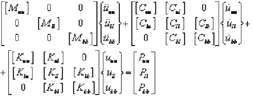
In this study, the bridge is model as 2D Euler-Bernoulli beam elements (Fig. 1). Each element includes four degrees of freedom, two for vertical deflections and the another two for nodal rotations. The equations of motion of the system can be express as in Eq. (2.1)
(1)
Fig. 1: Euler-Bernoulli beam element
where andare the mass, damping, stiffness matrices of the bridge, respectively;
and
are the nodal accelerations, velocities and deflections, respectively; is the nodal external forces. Damping of the bridge is assumed to followed Rayleigh type and calculated as
(2)
where and are damping coefficients, depend on damping ratio (usually equal to 5% for steel and 3%
for concrete), and the first two natural frequency of the beam and , and given as
(3)
2.2. Vehicle Equations of Motion
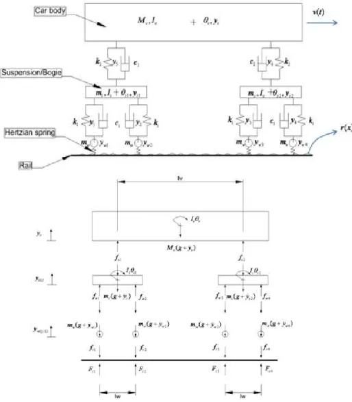
The vehicle is modeled as four-axle system, which consist a carbody supported by two bogies, and each bogie is suspended on two wheel axle as show in Fig. 2. The motion of the vehicle is represent as ten DOF, which includes bouncing and pitching of carbody and ; bouncing and pitching of two bogies
and ; and four bouncing at wheel axle . Among ten DOF, instead of four bouncing at wheel axles are constrained to the deflections of bridge, the other six DOF are unconstrained
Unconstrained DOF 〈 〉 (4)
Constrained DOF 〈 〉 (5)
Fig. 2: Vehicle model
Fig. 3: Free Diagram of Vehicle model
With this model, the free diagram can be expressed as in Fig. 3. The equations of motion of vehicle gives as follow:
(6) where andare the accelerations, velocities and deflections of the unconstrained degrees of freedom, and andare the accelerations, velocities and deflections of the constrained degrees of freedom. The corresponding sub-matrices of Eq.(6) are defined as Eq.(7)~Eq.(16)
(7)
(8)
(9)
(10)
(11)
(12)
(13)
(14)
〈 〉 (15)
〈 〉〈 〉 (16)
here and are the contact stiffness and contact forces at axle i; Q is the distributed weight of entire vehicle components at each axle. (17)
2.3. Hertzian Contact
There are many modification theories based on the original Hertzian theory. In this study, the most computational convenient adopted in [4] is used. Follow it, the Hertzian contact will be calculated as Eq.(18)
i f (18)
where is Hertzian contact coefficient, is the gap between wheel and rail.
2.4. Rail Irregularities
The wheel and rail will characteristic by power spectral density (PSD) functions. The irregularities may in periodic or no periodic. For the present purpose, in this study, the irregularities function has been adopted by [5] is used
exp
× sin
(19)
where x-along track distance (m); x0 = 1 m ; r0 = 0.5 mm – amplitude of irregularities; γ0 = 1 m wavelength of corrugation.
3. Derivation of the Coupled Equations of Motion
Fig. 4: Free Diagram of Vehicle model
Consider one wheel acting on element eth as show in Fig. 4. The load apply to the bridge will be
(20)
where yw ; yr is the deflection of mass Mv and bridge at contact point, r is the surface irregularity at contact point. Applying Hermitian interpolation function, the deflection of bridge at contact point yr can be computed from nodal displacements of acting beam element eth. Substituting to Eq.(20) and applies Hermitian functions for the forces we can obtains the nodal equivalent external forces when Mv moving between i and j is
(21)
or (22)
where {H} is Hermitian interpolation functions and defined as
(23)
and is the contact interpolation functions expressed as
(24)
Assembling by term Eq.(22) into bridge equations of motion, and adding vehicle degrees of freedom the equations of motion for the entire sysetem is
(25) Similarly, extending to 10 DOF vehicle model, the equations of motion of vehicle-bridge system can be expressed as
(26)
4. Numerical Examples
4.1 Simple Beam subjected to moving SprungMass
Consider a system as show in Fig. 4, where simple beam length L = 25 m, elastic modules E = 2.87 GPa, moment of inertial I = 2.90 m4, unit mass m = 2303 kg/m, mass Mv = 5750 kg k1 = 1595 kN/m, c1 = 0 travel with velocity of v = 27.78 m/s (100km/h).
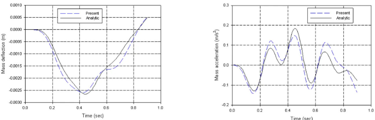
Using proposed program with the beam is modelled as 10 elements, integration time step is . The results are compared with the analytical results. The deflection and acceleration of midpoint of the beam are shown in Fig.5a and Fig.5b. The deflection and vertical acceleration of the mass are shown in Fig.6a and Fig.6b. As can be seen, very good agreements are obtained
(a) (b)
Fig. 5: Deflection and Acceleration of Midpoint of the Beam
(a) (b)
Fig. 6: Deflection and Acceleration of the Mass
4.2 Continuous Beam subjected to moving Train (KTX)
Consider a KTX train as show in Fig. 2, where simple beam length L=60m with three equal spans, E=2.825×10⁷kPa; I=495m4; A=373m2; mass per unit length 41.74t/m, neglect damping and rail irregularities.
Vehicle properties as Mv=54.960t; Iv=1131.9t.m2; ms=2.420t; Is=2.593t.m2; mw =2.048t; k1 = 2504kN/m; c1
= 32kN.s/m; k2 = 2536kN/m; c2 = 57kN.s/m. Moving with speed of v = 83.33m/s (300km/h).
(a) (b)
Fig. 7: Deflection and Acceleration of the Mass
(a) (b)
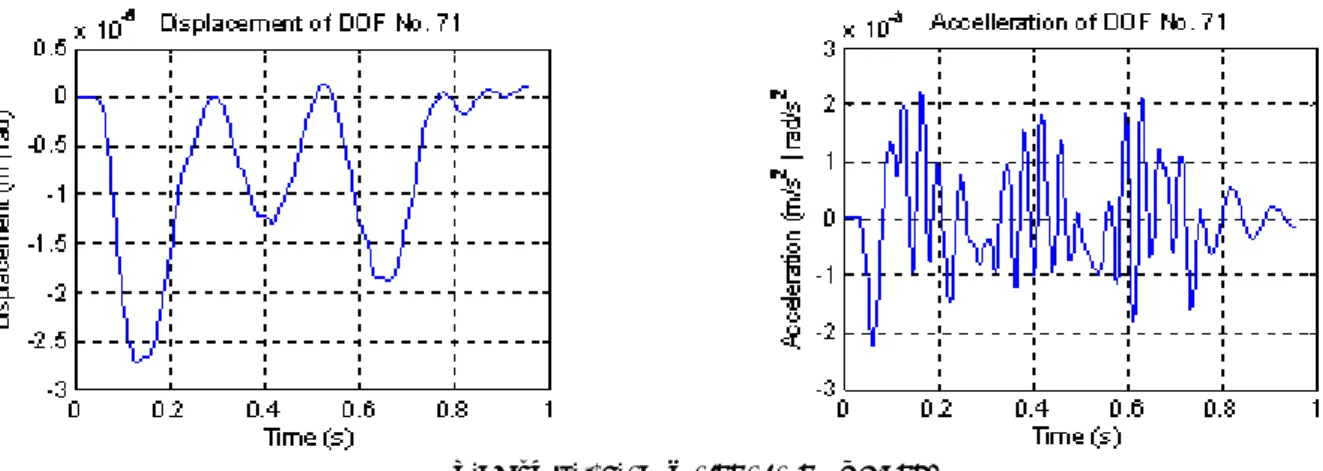
Fig. 8: Bouncing Response of Carbody
(a) (b)
Fig. 9: Pitching Response of Carbody
Using proposed program with the beam is modelled as 30 elements, integration time step is . The midpoint deflection of left span and centre span are plotted in Fig.7a and Fig.7b. The deflection and acceleration of bouncing responses of carbody is plotted in Fig.8a and Fig.8b. The deflection and acceleration of pitching responses of carbody is plotted in Fig.9a and Fig.9b
5. Conclusion
In this study, the coupled equations of motion for the entire vehicle-bridge system is derived including Hertzian contact and rail irregularities. The convenient formulas are encoded into a computer program. The accuracy and efficiency of the proposed program is verified with the exact analytical results, and a good agreement are obtained. As a result, the proposed program is applied to analysis the response of real KTX train, all responses of bridge and vehicle are investigated.
Acknowledgment
This work was supported by the Korea Science and Engineering Foundation (KOSEF) grant funded by the Korea government (MEST) (No.R0A-2005-000-10119-0).
References
1. Dukkipati, R.V. and V.K. Garg, Dynamics of Railway Vehicle Systems. 1984, Canada: Academic Press.
2. Wu, J.-S. and P.-Y. Shih, Dynamic Responses of Railway and Carriage under the High-Speed Moving Loads. Journal of Sound and Vibration, 2000. 236(1): p. 61-87.
3. Lei, X., Dynamic analysis of the track structure of a high-speed railway using finite elements. Proceedings of the Institution of Mechanical Engineers, Part F: Journal of Rail and Rapid Transit, 2001. 215(4): p.
301-309.
4. Shabana, A.A., K.E. Zaazaa, and H. Sugiyama, RAILROAD VEHICLE DYNAMICS: A computational approach. 2008: CRC Press.
5. Nielsen, J.C.O. and T.J.S. Abrahamsson, Coupling of Physical and Modal Components for Analysis of Moving Non-linear Dynamic Systems on General Beam Structures. International Journal for Numerical Methods in Engineering, 1992. 33(9): p. 1843-1859.