A study on Defect Diagnosis of Gas Turbine Engine Using Hybrid SVM-ANN in Off-Design Region

A study on Defect Diagnosis of Gas Turbine Engine Using Hybrid SVM-ANN in Off-Design Region

Dong-Hyuck Seo, Won-Jun Choi, Tae-Seong Roh, Dong-Whan Choi Aerospace Department – Inha University

253 Yonghyun-Dong Nam-Gu Incheon 402-571 Republic of KOREA [email protected] [email protected]

Keywords: Gas Turbine, Defect Diagnosis, Support Vector Machine, Artificial Neural Network Abstract

The weak point of the artificial neural network (ANN) is that it is easy to fall in local minima when it learns too much nonlinear data. Accordingly, the classification ratio must be low. To overcome this weakness, the hybrid method has been proposed. That is, the ANN learns data selectively after detecting the defect position by the support vector machine (SVM).

First, the SVM has been used for determination of the defect position and then the magnitude of the defect has been measured by the ANN. In off-design condition, the operation region of the engine is wide and the nonlinearity of learning data increases. The module system, dividing the whole operating region into reasonably small-size sections, has been suggested to solve this problem. In this study, the proposed algorithm has diagnosed the defects of triple components as well as single and dual components of the gas turbine engine in off-design condition.

Introduction

For safe operation of an aircraft, researches about the diagnosis system of gas turbine engine to increase maintenance economical efficiency have been active recently. The defect diagnosis system generally measures the performance parameter such as pressures, temperatures across each component and analyzes a certain tendency, then determines whether the engine is healthy or not.^1,5) The early detection and prediction of engine defect have much benefit such as preventive maintenance, reduction of maintenance cost and time.

It can also increase stability and reliability of an aircraft in flight.

Generally, the artificial neural network (ANN), the generic algorithm (GA) and the support vector machine (SVM) have been utilized to develop the defect diagnosis system¹⁾. The ANN algorithm is able to predict the characteristics of uncertain groups based on the specific information. The GA is a way of solving problems by mimicking the same processes which nature uses. The GA uses the combination of selection, recombination and mutation to evolve a solution of a problem. The SVM which is able to classify and analyze the pattern with fewer data is functional and efficient method⁸⁾.

In this paper, the SVM and the ANN algorithms have been used as a defect diagnosis system. The ANN algorithm has been widely used to solve the pattern recognition problem of the defect diagnostic

system.³⁾ However, this tool has many weak points;

it’s too hard to know the ending time of learning, moreover the most serious problem is the possibility of falling in the local minima. Because of these weak points, it becomes very difficult to obtain good convergence ratio and high accuracy. To solve these problems, the hybrid SVM-ANN method has been suggested. The SVM has been applied as a sorter of the defect location accompanied with an enormous amount of data, and then the ANN algorithm has been applied to estimate the defect magnitude. This hybrid method has advantages of the reducing of learning data and converging time without any loss of estimation accuracy, because the SVM classifies the defect location and reduces the learning data range.

In off-design condition, the operation region of the engine is much wider. Accordingly the number of learning data is more enormous. So, the nonlinearity of learning data increases considerably and the performance of the hybrid method become non- efficient. To solve the problem, a module system has been suggested. The module system is that the whole operating region is divided into reasonably small-size section.

In this work, the proposed hybrid SVM-ANN with the module system algorithm has diagnosed triple defects as well as single and dual defects of 3 major components (the compressor, the gas-generator turbine, the power turbine) of gas turbine engine in whole off-design region. As results, it has been shown that the real-time diagnosis for the single and multiple defects in whole off-design region be possible, and the hybrid SVM-ANN method with the module system has reliable and suitable defect estimation accuracy.

Fig.1 Hybrid method of SVM and ANN Submit all data sets to SVM

Lean all class data

Classify the class of the test data

Class 1 Class 2 Class 3 Class 4

ANN Defect Magnitude

The Hybrid Method

Structure of Hybrid method

All data has been classified to several classes by SVM. The magnitude of classified data has been measured by ANN. Fig. 1 shows the structure of hybrid method.

For example, suppose that “Class1” is the compressor defect group, and if the defect occurred in the compressor, the SVM algorithm classifies

“Class1” of whole classes. Then, the ANN algorithm measures the defect magnitude with only compressor data which is classified by SVM.

Support Vector Machine

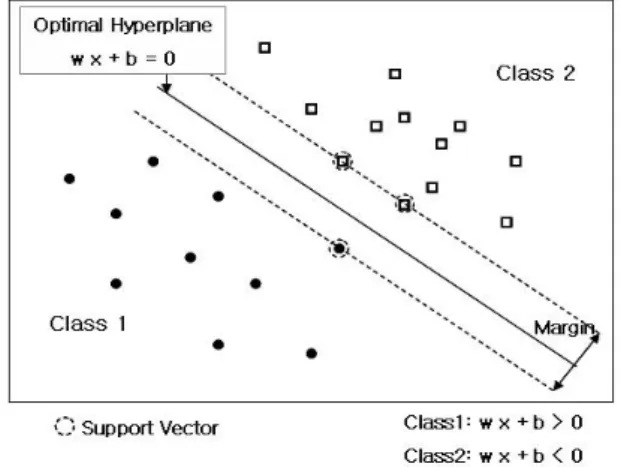
The purpose of SVM presumes the hyper-plane which classifies learning data in two classes. There are many possible planes, but only one plane is shown to maximize the margin among the classes viewed by fig.

2^11,12). This plane is the optimal hyper-plane to serve as the binary sorter.

Fig. 2 Optimal hyper-plane and support vector To obtain the maximum margin, first Lagrange multiplier α_i must be calculated by the QP solver.

Using Eq. (1) and Eq. (2), the hyper-plane equation b

x

w⋅ + can be obtained. Finally, the decision function Eq. (3) with the hyper-plane equation is utilized for classifying the class including arbitrary vectorx.

∑

∑

=

=

i i i N

i

i i

iyx yx

w α α

1

(1)

1 ) ) (

(

∑

∈

b x x y y

SV i

i i i i

i α (2)

) ((

) , ,

(x a^* b^* sign w^* x b^*

f = ⋅ +

) ) ( (

∑

∈

+

⋅

=

SV i

i i

iy x x b

sign α (3)

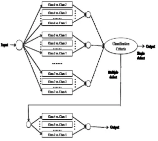
To increase the classification accuracy of the nonlinear data, Gaussian Kernel Function has been used. The SVM algorithm has been expanded to

multi-class SVM, especially “One vs. One”, to classify the multiple groups. Figure.3 shows the form of “One vs. One” multi-class SVM suggested by Clarkson and Moreno⁵⁾.

Fig. 3 One vs. One Multi-Class SVM Classifier Artificial Neural Network

The organized neural network used the multi-layer perceptron as the most general form has been applied for the error back propagation algorithm. Figure 4 shows the structure of ANN.⁷⁾

Fig. 4 Structure of ANN model

The information from the input-layer is multiplied by weights and biases before it is transferred to the hidden layer. In a similar method, the calculated information of the hidden-layer is delivered to the output layer. The ANN output (O_pk) is computed in this process. Consequently, the error between the ANN output and the desired output (d_pk ) are as follow;

∑∑

∑

=

−

=

=

p M

k

pk pk p

p d O

E E

1

1

)2

2 (

1 (4)

To make this error be the least, weights are changed as follow;

kj kj

kj W

t E W t

W ∂

− ∂

=

+1) ( ) η

( (5)

This process is repeated until the error is satisfied with the convergence condition. The weights and biases as the calculation results are stored to estimate the state of new data.

The momentum theory13) has been used to promote convergence of the ANN and the sigmoid function^7,14) used to classify nonlinear input pattern has been applied as Eq. (6) below.

e bx

x

f ₋

= + 1 ) 1

( (6)

Advanced Hybrid Method in Off-design region In off-design condition, the number of learning data is enormous and then the nonlinearity of data also increases. Therefore, it is necessary to reduce the size of learning data.

If the general SVM diagnoses the defect location, the classification time, especially in triple defect case, increases considerably. So, the real-time estimation becomes almost impossible. To reduce the running time of the SVM method, additional idea must be suggested. The advanced SVM method has the classification of two steps. At the first step, the “One vs. one” SVM classifies the defect position of single defect and multiple defects without distinguishment of dual defects and triple defects. At the next step, the multiple defects are classified as the dual defects and the triple defects by using the SVM again. If the classified data has any defect at the last step, this state is the case of the triple defects. The structure of the advanced SVM method has been shown as Figure. 5.

Fig.5 Advanced Multi-SVM Structure

The ANN learning data in the off-design region has been divided by the altitude and the data divided by the altitude are also divided by the fuel mass flow rate and the Mach number. Accordingly, the size of learning data is larger than at sea-level condition and convergence ratio of data increases. Therefore, the convergent ratio of the ANN method becomes poor.

This problem can be solved by the Module system. In the module system, the data of whole off-design

region are not necessary to be learned. The data only near the region where the defect is diagnosed are needed to learn. That is, Module system is that the whole operating region is divided into reasonable small-size sections. Figure 6 shows the structure of the module system.

Fig. 6 Hybrid method with Module system

Application

Engine selection and modeling

In this study, the suggested algorithm has been applied to a turbo-shaft engine. On-design and off- design performance data of the engine have been generated by a gas turbine simulation program (GSP).

The characteristic maps of the centrifugal compressor and the turbine maps, which are provided by GSP, have been scaled for our own purpose.

The major parts to estimate the engine state are the compressor, the gas-generator turbine and the power turbine. Therefore, single and multiple defects with the components are considered. Class 1 is a reference state. Class 2~4 represent a single defect state of each component. And class 5~7 represent a dual defect state of two components. Finally class 8 represents a triple defect state of all components. (Table 1)

Table 1 Class Classification by Defect position Class no. 1 2 3 4 5 6 7 8

Defect no. 0 1 2 3

Compressor

GG- Turbine P-Turbine

As the input data of the defect diagnostic algorithm, the temperatures cross all parts and the pressures across the compressor have been obtained by GSP.

The isentropic efficiency of each part has been used to

estimate whether the engine has a defect, or not.

(Table 2)

Table 2 Input Data and Output data of hybrid method

Input Output

Hybrid Method

Compressor ^t2

T , T_t3

2

Pt , P_t3 η^c

GG-Turbine T_t4, T_t7 η_ggt

P-Turbine T_t7, T_t8 η_pt

Applying the hybrid method to off-design condition The hybrid method has been applied to the off- design condition. For data learning, the section of data has been divided into the altitude, the Mach number and the fuel flow rate. The altitude has been divided into 21 sections from the sea level (0 m) to maximum operating altitude 4,800 m. Each altitude data includes variation of the velocity and the fuel flow rate. The ranges of the Mach number and the fuel flow rate are 0~0.5 and 0.030~0.038 kg/s, respectively. To simulate the engine with the defects, the forced defect has been applied to the learning data. The forced defect has been represented by minus isentropic efficiency in GSP. The defect rate is 0.0~-5.0%.

Table 3 Input Data for learning on Off-design

Defect Location Alt.

(m)

Mach no.

Fuel flow rate

Forced defect magnitude Compressor( C )

0, 240,

~ 4,800

0.0

~ 0.5

0.030 kg/s

~ 0.038

kg/s

-0.5 % -1.0%

~ -5.0%

GG- turbine( GGT ) P-turbine ( PT )

C+GGT C+PT GGT+PT All components

According to each altitude and Mach number, the fuel flow rate must be deferent in all cases. If same fuel flow rate are used in all cases, the fuel lean or rich combustion is appeared in a specific altitude. Table3 shows the input data for learning on off-design condition.

To confirm the reliability of algorithm, the test data is required. The test data has been selected arbitrarily between continuous learning data. Each test data has 3 Mach No. condition; 0.1, 0.2, 0.4. The test data is obtained by GSP. (Table 4)

Decision of defect position

The general SVM has been utilized to detect single or dual defects. All data are classified 100% as shown in Table 5. The average convergence time for defect

predictions is about 36 seconds per case. The convergence time of triple defect case is, however, about 1,400 sec.

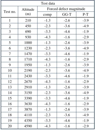
Table 4 Test data

Test data

Test no. Altitude (m)

Forced defect magnitude comp GG-T P-T 1 210 -1.3 -2.6 -3.9 2 450 -2.3 -3.6 -4.9 3 690 -3.3 -4.6 -1.9 4 930 -4.3 -1.6 -2.9 5 1000 -1.3 -2.6 -3.9 6 1230 -2.3 -3.6 -4.9 7 1470 -3.3 -4.6 -1.9 8 1710 -4.3 -1.6 -2.9 9 1950 -1.3 -2.6 -3.9 10 2190 -2.3 -3.6 -4.9 11 2430 -3.3 -4.6 -1.9 12 2670 -4.3 -1.6 -2.9 13 2910 -1.3 -2.6 -3.9 14 3150 -2.3 -3.6 -4.9 15 3390 -3.3 -4.6 -1.9 16 3630 -4.3 -1.6 -2.9 17 3870 -1.3 -2.6 -3.9 18 4110 -2.3 -3.6 -4.9 19 4350 -3.3 -4.6 -1.9 20 4590 -4.3 -1.6 -2.9

To solve this problem in case of triple defect diagnosis, the advanced SVM has been used. This advanced method classifies 100% and convergence time is about 36 sec.

Table 5 SVM classification results

Estimation of defect magnitude

The defect data group classified by the SVM has been estimated by the ANN. The ANN estimates the defect magnitude by learning the temperature ratio and the pressure ratio at specific condition such as the altitude, Mach number and the fuel flow rate obtained in real-time. The ANN learning through the sensed parameters of whole off-design is executed at the sea- level and the weight and bias obtained from the

Defect position

Classification Accuracy

General Advanced Average convergence

time

C 100 %

36 s 36 s GGT 100 %

PT 100 % C+GGT 100 %

C+PT 100 % GT+PT 100 %

C+GT+PT 100 % 1400 s 36 s

learning are used on flight for defect diagnosis in real- time.

The RMS defect error rate calculated at each altitude has been used to estimate algorithm reliability.

It means the percentage of the difference between the real defect and the calculated defect values. It is defined as below

= ∑

=

− ×

N

i

i real

cal

real N

D D D

1

2/

%) 100

( (7)

Each test data, which is used to compare real-values and calculated values, has been divided by the fuel flow rate and Mach number. The fuel flow rate is divided into 0.032kg/s and 0.038kg/s. And Mach number is divided into 0.1, 0.2 and 0.4. The defect magnitudes of single or multiple defects are shown at Table 4.

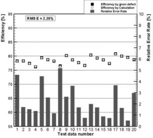
Fig. 7 Estimated efficiency and Relative Error rate of compressor

Fig. 8 Estimated efficiency and Relative Error rate of GG-turbine

Fig. 9 Estimated efficiency and Relative Error rate of Power turbine

Figure 7, 8 and 9 show the efficiency and the relative error rate of single defect. The square symbol filled with black means the efficiency by the given defect and the diamond symbol means the calculated efficiency (The left side of y-axis). The relative error rate of each test case is expressed by a bar graph. (The right side of y-axis) The x-axis is test number. In single defect diagnosis, the RMS defect error rates of each component (Compressor/GG-Turbine/Power Turbine) are 2.28% / 3.54% / 2.89%.

Figure 10, 11 and 12 show the dual defect cases.

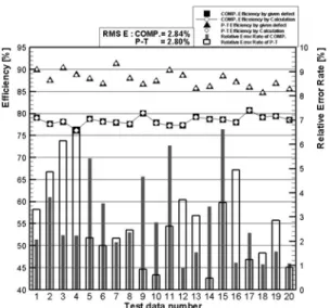
Each figure shows the multiple defects of compressor and G-G turbine / compressor and power turbine / G- G turbine and power turbine. In the same manner as single defect, the triangle and square symbol filled with black represent real-efficiency. The diamond and a polygonal line with diamond represent calculated efficiency. In dual defect diagnosis, the RMS defect error rates of each case (compressor/G-G turbine, compressor/power turbine, G-G turbine /power turbine) are 3.11% / 2.84%, 2.84% / 2.80% and 2.30%

/ 3.62%, respectively.

Fig. 10 Estimated efficiencies and Relative error rate of Compressor and GG-Turbine

RMS defect error rate

Fig. 11 Estimated efficiencies and Relative error rate of Compressor and Power Turbine

Fig. 12 Estimated efficiencies and Relative error rate of GG-turbine and Power Turbine

Figure 13, 14 and 15 show the triple defect case.

The triple defects are estimated by using the hybrid method with the module system. The RMS defect

Fig. 13 Estimated efficiencies and Relative error rate

of Compressor in 3 components defect case

error rates are 3.68% / 1.28% / 2.79% for the compressor / G-G turbine / power turbine, respectively.

Fig. 14 Estimated efficiencies and Relative error rate of GG-Turbine in 3 components defect case

Fig. 15 Estimated efficiencies and Relative error rate of Power Turbine in 3 components defect case At Table 6, non-module and module learning of the defect mean error have been compared at 1,000m. For the single defect case, the defect error rates have decreased from 12.55% to 4.47% at the compressor, from 16.54% to 6.16% at the G-G turbine and from 20.21% to 2.05% at the power-turbine. For the dual defect case, the defect error rates have decreased from 37.61%/9.08% to 4.04% /3.25% at compressor/G-G turbine, from 31.91%/44.27% to 8.48%/2.16% at compressor/power turbine and from 17.82%//33.29%

to 2.19% //3.09% at G-G turbine/power turbine. Also, for triple defects case, the defect error rates have decreased from 39.92%/9.06%/107.49% to 7.24%

/0.79%/2.83% at compressor/G-G turbine/Power Turbine. The results have shown the estimated accuracy of the hybrid SVM-ANN with the module system is far better than that of general hybrid SVM- ANN method.

Table 6 Comparison of the defect mean error rate of non-module and module learning of hybrid method

Defect mean error rate (%) Learning of all data

For 1,000m

Learning of one module for 1000m

C 12.55 4.47

GG-T 16.54 6.16

P-T 20.21 2.05

C/GG-T 37.61 9.08 4.04 3.25 C/P-T 31.91 44.27 8.48 2.16 GG-T/P-T 17.82 33.29 2.19 3.09

All components

C GG-T P-T C GG-T P-T

39.92 9.06 107.49 7.24 0.79 2.83

Conclusion

In this study, the hybrid SVM-ANN method with module system has been proposed for defect diagnosis of the aircraft gas-turbine engine.

The SVM has been utilized for detecting defect location as a classifier. Especially, the advanced SVM, which has one more classifier to find the locations of the dual defects and the triple defects, has been used to classify the multiple defects as well as the single defect. This method helps to reduce the convergence time for real-time diagnosis.

The ANN has been used to estimate the defect magnitude. The learning data in off-design condition, however, increase the non-linearity of the input data.

So, the module system has been proposed to decrease non-linearity. The learning data of whole off-design region are divided into appropriate-size sections, which is module concept. To estimate the defect of arbitrary point, the learning data of specific module including the point is used.

The proposed algorithm, the hibrid SVM-ANN method with the module system, has diagnosed the defects of triple components as well as the single and the dual components of the gas turbine engine in off- design condition. As the results, the real-time diagnosis for the single and the multiple defects in whole off-design region shows reliable and suitable accuracy of the defect estimation.

References

1) Link C. Jaw, "Recent Advancements in Aircraft Engine Health Management (EHM) Technologies and Recommendations for the Next Step", 50th ASME International Gas Turbine & Aeroengine Technical Congress, 2005

2) HU Zhong-hui, CAI Yun-ze, LI Yuan-gui, and XU Xiao-ming, "Data fusion for fault diagnosis using multi-class Support Vector Machines,"

Journal of Zhejiang University Science, 2005, Vol.6A, no.10, pp. 1030~1039

3) Stanislaw Osowski, Krzysztof Siwek, Tomasz Markiewicz, "MLP and SVM Networks - a Comparative Study," Proceedings of the 6th Nordic Signal Processing Symposium - NORSIG, 2004

4) Takahisa Kobayashi, Donald L. Simon, Takahisa Kobayashi, "A Hybrid Neural Network-Genetic Algorithm Technique for Aircraft Engine Performance Diagnostics", NASA/TM-2001- 211088, 2001

5) Xuechuan Wang, "Feature Extraction and Dimensionality Reduction in Pattern Recognition and Their Application in Speech Recognition,"

Ph.D. Thesis, 2002, pp.86~89

6) R.B.Joly, S.O.T. Ogaji, R.Singh, S.D. Probert,

"Gas-turbine diagnostics using artificial neural- networks for a high bypass ratio military turbofan engine", Applied Energy Vol.78, no.4, 2004, pp.397~418

7) Parag C. Pendharkar, "A data mining-constraint satisfaction optimization problem for cost effective classification", Computers & Operations Research Vol.33, no.11, 2006, pp. 3124~3135 8) A Gammermann, "Support vector machine

learning algorithm and transduction,"

Computational Statistics, Vol. 15, No. 1, 2000, pp.31~39

9) Sheng-Fa Yuan, Fu-Lei Chu, "Support vector machines-based fault diagnosis for turbo-pump rotor", Mechanical Systems and Signal Processing Vol.20, no.4, 2006, pp.939~952

10) K. Schittkowski, "QL: A Fortran Code for Convex Quadratic Programming - User's Guide, Version 2.1", University of Bayreuth , 2004 11) Christopher J. C. Burges, “A Tutorial on

Support Vector Machines for Pattern Recognition,” Kluwer Academic Publishers, Boston, pp.1-433

12) Ming Ge, R. Du, Guicai Zhang, and Yangsheng Xu, “Fault diagnosis using support vector machine with an application in sheet metal stamping operations,” Mechanical System and Signal Processing, Vol.18, 143-159, 2004

13) Vijay S. Mookerjee, Michael V. Mannino,

“Sequential Decision Models for Expert System Optimization”, IEEE Transactions on knowledge and data engineering, Vol. 9, No. 5, 1997

14) B. Samanta, K. R. Al-Balushi, and S. A. Al- Araimi, “Artificial neural networks and support vector machines with genetic algorithm for bearing fault detection,” Engineering Application of Artificial Intelligence, Vol.16, pp.657-665, 2003

Acknowledgments

This study has been performed as a part of the Smart Unmanned Air Vehicle (SUAV) development program. This work has been supposed by the Ministry of Commerce, Industry and Energy (MOCIE) and the Korea Aerospace Research institute (KARI).

Appendix

Nomenclature

b = Standard vector of hyper-plane

dpk = desired output of k row

Dreal = Real defect magnitude

Dcal = Calculated defect magnitude

E = Cost Function error value GG-T = Gas Generator Turbine

N = Data set number

Opk = Objective output of k row

P-T = Power turbine

Pt = Total pressure

Q = Lagrange objective function

Tt = Total temperature

w = Direction vector of hyper-plane

Wkj = kjth connection intensity of neuron

y = Labels

α = Lagrange Multiplier

η = Isentropic efficiency Subscript

c = Compressor

ggt = Gas generator turbine pt = Power turbine

2

t = Compressor inlet

3

t = Combustor inlet

4

t = Gas generator turbine inlet 7

t = Power turbine inlet 8

t = Power turbine outlet