https://doi.org/10.7848/ksgpc.2016.34.6.569
Development of Realtime GRID Analysis Method based on the High Precision Streaming Data
Lee, HyeonSoo
1)· Suh, YongCheol
2)Abstract
With the recent advancement of surveying and technology, the spatial data acquisition rates and precision have been improved continually. As the updates of spatial data are rapid, and the size of data increases in line with the advancing technology, the LOD (Level of Detail) algorithm has been adopted to process data expressions in real time in a streaming format with spatial data divided precisely into separate steps. The existing GRID analysis utilizes the single DEM, as it is, in examining and analyzing all data outside the analysis area as well, which results in extending the analysis time in proportion to the quantity of data. Hence, this study suggests a method to reduce analysis time and data throughput by acquiring and analyzing DEM data necessary for GRID analysis in real time based on the area of analysis and the level of precision, specifically for streaming DEM data, which is utilized mostly for 3D geographic information service.
Keywords : LOD (Level of Detail), High Precision Streaming, DEM, Realtime Grid Analysis
569 Original article
Received 2016. 11. 23, Revised 2016. 12. 08, Accepted 2016. 12. 31
1) Dept. of Civil Engineering, Pukyong National University, Korea (E-mail: [email protected])
2) Corresponding Author. Member, Dept. of Civil Engineering, Pukyong National University, Korea (E-mail: [email protected])
This is an Open Access article distributed under the terms of the Creative Commons Attribution Non-Commercial License (http://
creativecommons.org/licenses/by-nc/3.0) which permits unrestricted non-commercial use, distribution, and reproduction in any medium, provided the original work is properly cited.
1. Introduction
Since the beginning of the 21st century, we have witnessed a dramatic increase in the number and the quality of information as much of the information throughout the world goes online thanks to the development of the Internet and electronic devices. With the development of IT (Information Technology) and smart devices, spatial information, which was previously used mainly in the government, public organizations, corporations and academies, has been gradually utilized as personal spatial information as it is integrated with private information. Against such backdrop, IT companies that provide customized services have also
developed spatial information technology that enables people to use more high-precision and high-speed services. As the amount of spatial information accumulates over time, its data volume increases faster than the speed of equipment and communications which process the data. However, users want faster reactivity in using high-precision spatial information given by new technologies such as augmented reality, virtual reality, or IoT (Internet of Things). Therefore, researchers have promoted the development of technologies that can accurately deliver large-scale, large-capacity spatial information with smaller transmission volume and processing capacity.
In the past, researchers created contour-based
Journal of the Korean Society of Surveying, Geodesy, Photogrammetry and Cartography, Vol. 34, No. 6, 569-578, 2016
570
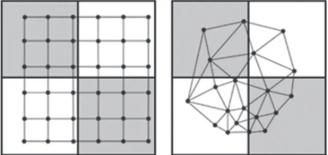
topographic maps in a form of TIN (Triangular Irregular Network) through the terrain elevation for the analysis of the grid unit at first (Choi and Yoon, 1994; Cho, 1999); and secondly, used Bspline interpolation methods to create a raster map of the average elevation based on grid (Fig. 1).
Then, the researchers analyzed elevation information of the horizontal plane based on the elevation information of Raster data in which the elevation points are arranged at the same interval in order to perform an analysis of the terrain on the basis of grid such as slope and aspect of the terrain (Yoon, 1998; Nam, 2002). Previously we used the digital topographic map at a scale of 1: 1000 or more. But thanks to development of measuring devices, now it has become possible to increase the accuracy and enhance analysis process as the equipment like LiDAR outputs the grid-based DEM data with an elevation gap of less than 1 m. However, consequently, as the precision level increases, and the areas of DEM becomes larger, the original data produced by the high-precision DEM data has highly bigger volume, thereby consuming more time during the course of pre-processing the information for analysis.
Therefore, in this research, we started from the research that visualizes the DEM data of high precision and large capacity in real time. We collected a small unit of DEM data required for analysis in the same way and analyzed the collected DEM data by DEM unit through topographic analysis algorithm. Since very small units of data come for streaming, the elapsed time for the analysis is very short while its results can be shown immediately. Therefore, we suggest this analysis method of the terrain and space as a way of analyzing in real-time and visualizing them.
For the real-time terrain analysis, we utilized the DEM
data from the VWorld, a spatial information open platform which is created and distributed by the Ministry of Land, Infrastructure and Transport as for high precision, streaming DEM data in this research.
2. Research Methods
For grid analysis, it is necessary to extract the data required for the analysis in order to standardize and quantify the analysis. This sample information differs depending on the type of the terrain model forming the terrain as shown in Fig. 2. Since the terrain model created by a vector method such as contour lines or TIN has a spatially irregular elevation reference point, the variation range becomes bigger as to the number of elevation reference points extracted in the unit space of the grid. It is a general trend to perform the grid analysis after interpolating as DEM data in a Raster type with standardized terrain elevation point in this direction.
2.1 DEM with LOD algorithm
As for DEM, its data size is decided in proportion to the gird space, the precision level of elevation value and spatial size. And in the case of the high-precision, large-scale DEM, since the scope and the quality of expression should be decided in visualizing all DEM data after bringing them at once, the LOD (Level of detail) algorithm is applied to create the expression level by step. And in order to stream the data at each step's level, researchers apply regular expressions to create unit data with the same density and establish data system that allows to find only necessary information through Fig. 1. The process of converting a contour line model to a
raster height model
Fig. 2. Height value detected in the terrain model
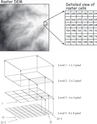
571 spatial indexing (Bryan, 2000). Since the DEM data takes
the Raster type, researchers use such characteristics: apply the Gaussian pyramid algorithm that is used in the image processing for accelerated image visualization in order to repeat the process of reducing the precision level step-by- step. As such steps are repeated, researchers create the DEM data of a pyramid type with phased precision degrees where the range of the data gradually increases while the density becomes lower. Accordingly, they maintain the consistency of data by shifting the DEM of the area to be used from the low precision to the high precision sequentially (Lee et al., 2009).
Fig. 3. Gaussian Pyramid application example In order to calculate the value of the upper table in case of going up to the upper level, researchers use the following formula Eq. (1) to have the interpolation value of the upper level DEM terrain elevation from the Gaussian Pyramid algorithm (Fig. 3).
where column index number
row index number
Denote the Value on level
(2)
deg
×
[
] [
]
(1)
where
where column index number
row index number
Denote the Value on level
(2)
deg
×
[ ] [ ]
×
+g)
×
column index number
where column index number
row index number
Denote the Value on level
(2)
deg
×
[
] [
]
× +g)
×
row index number
Denote the Value on
where column index number
row index number
Denote the Value on level
(2)
deg
×
[ ] [ ]
×
+g)
×
level where column index number
row index number
Denote the Value on level
(2)
deg
×
[ ] [ ]
× +g)
×
2.2 DEM data in a tiling method and spatial index
The high-precision DEM data, which is made up of one huge data form, requires a lot of time from the process of loading it, and since all the data must be stored in the process of selecting and processing the data to be actually used, the memory usage rate of the storage medium and the system becomes very high. To solve this problem, it is necessary to collect and process quickly only small data from the necessary area. In order to be able to calculate spatial indexing faster than simply dividing the data into pieces, the DEM data is separated into division of the space by step and tile-based classification. Then, researchers load the data as unit data, thereby realizing indexing of the space at a high speed through unique identification number (Stefan et al., 1998).
The data used in this research is VWorld DEM data from the open platform for space information, and according to the criteria for selection, the platform is available for all and has the DEM with 5m grid spacing, which is most precise based on the Korean Peninsula (90m in the world, 1km below the sea level), under the condition of tiled high precision DEM data for streaming. The VWorld uses NASA's World Wind Map Tile System in order to implement tiling for streaming.
The Map Tile System is mainly classified into two types.
The most commonly used one is Quardtree Tile System
through Mercator Projection such as MS Bing Map, Google
Map, Open Street Map, etc. which the whole earth is divided
into four sections with the lower tiles and is mainly used for
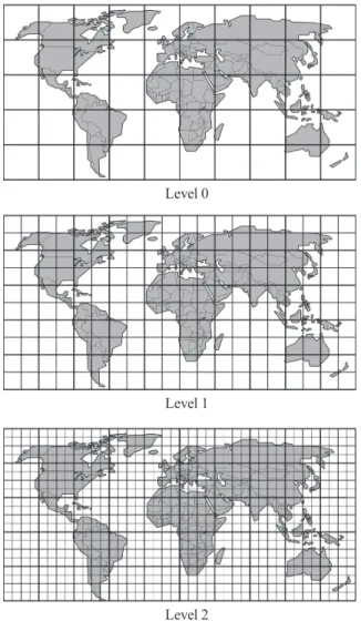
two dimensional maps. As for the NASA World Wind, the
earth spherical body is divided into 10 longitude zones and
five latitude tile zones by dividing the longitude and latitude
by 36 degrees respectively. This method is usually used
in three dimensional maps, and these tile zones are again
divided into the longitude and latitude by two respectively,
creating the lower level tiles (Fig. 4).
Journal of the Korean Society of Surveying, Geodesy, Photogrammetry and Cartography, Vol. 34, No. 6, 569-578, 2016
572
Level 0
Level 1
Level 2
Fig. 4. Grid size of world wind map tile system With such configuration, the spatial index moves along with the x-axis and the y-axis towards the upper right direction based on the lowest left end of the tile. (Fig. 5)
The data of each tile unit is all divided into files based on the spatial index, and as a result, the data is loaded (Fig. 6).
Fig. 6. Examples of store spatial data
3. Implementation Methods
3.1 Specification of VWorld DEM data
When it comes to the VWorld's DEM data, each tile's width and height have 36 degrees of latitude and longitude degree at the 0 level. The level 1 is reduced by half angle to 18 degrees, and the level 2 is to nine degrees, and so forth. In addition, one tile has 65 altitude reference points in each of the horizontal and vertical directions, forming 64 lattices in width and height respectively (Fig. 7).
At the n-level, each lattice's horizontal and vertical spacings are calculated as Eq. (2), and the number of DEM Fig. 5. Example of zero level index coordinates
Fig. 7. Index coordinates of altitude reference point of
DEM data
Development of Realtime GRID Analysis Method based on the High Precision Streaming Data
573 lattice is 4096.
where column index number
row index number
Denote the Value on level
(2)
deg
×
[ ] [ ]
×
+g)
×
(2)
The DEM elevation reference point of the VWorld consists of the floating point number of a 32-bit single-precision and has 23 bit as mantissa. Since the elevation reference point has the same number for all tiles, it has the following values:
where column index number
row index number
Denote the Value on level
(2)
deg
×
[
] [
]
×
+g)
×
As for the elevation of each lattice, calculate the height of the elevation by averaging the four elevation reference points that surround the lattice.
3.2 Analysis procedure
Fig. 8. Comparison of previous and presenting The previous analytical model requires all the data and prepares and processes the analysis for a long time. On the other hand, the proposed analysis model takes a short time to prepare and process the analysis in units. The analysis is completed by repeating the process. (Fig. 8)
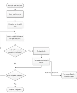
This research followed the below process. The researchers of this study realized the main processing to analyze the space by inputting the area for geographical grid analysis, extracting the list of necessary unit DEMs through spatial indexing of the relevant area and applying the grid analysis algorithm based on this unit DEM (Yoon, 2007). We developed a loading method which enables to visualize such analyzed results and at the same time, to load the results
to a comprehensive analysis database for the extraction of statistical results (Fig. 9).
Fig. 9. Grid analysis processing flowchart
3.3 Grid analysis area input and the precision level setting
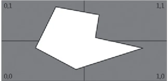
We input the analysis area for analysis in order to perform the grid analysis and set up the relevant limit analysis area and the analysis precision level. In terms of the limit analysis area, we calculated the limit analysis area comprising the MBR (Map Bound Rect) in the analysis area and limiting the scope of the DEM data within the calculation area (Fig.
10). Moreover, since the DEM used in this research is the one
where the LOD is applied, we reflected the part that enables
to select the precision level to control the accuracy of the time
and results of the analysis. In this research, we used the LOD
level coefficient for the accuracy calculation. It is possible
to obtain a precise elevation reference point with a small
number of the LOD interpolation as the level coefficient
increases, the total number of unit DEMs required for the
same area increases, thereby taking more time for analysis
and narrowing the space of the elevation reference point of
the DEM (Figs. 11 and 12).
Journal of the Korean Society of Surveying, Geodesy, Photogrammetry and Cartography, Vol. 34, No. 6, 569-578, 2016
574
3.4 Division of the grid areas and spatial indexing calculation
As for calculation of analysis area and the precision level, we need to calculate spatial indexing in order to collect the related DEM data. To calculate based on the analysis area, we calculated the minimum and the maximum latitude and longitude coordinates of the analysis area so that we can calculate the x-axis column and the y-axis row included in the relevant areas.
In terms of the longitude, we created the x-axis index number column ID by dividing the longitude entered on the x-axis that extends up to 360 degrees on the basis of 0 degree
Fig. 10. DEM expanding over the analysis area of the N level
by the lattice spacing. In terms of the latitude, we calculated the y-axis index number row ID by dividing the latitude entered on the x-axis that extends up to 90 degrees starting from -90 degrees by the lattice spacing (Fig. 13).
The limit analysis area refers to the maximum and the minimum ranges of column ID and row ID, and the DEM included within this ID range is selected as a priority (Fig.
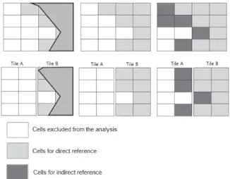
14). We created a process to differentiate the area for analysis by checking whether it affects the polygon of analysis area and the unit grid from the selected area (Fig. 15).
Fig. 13. The analysis area is expanded on tiles
Fig. 14. Calculating the limit analysis area
3.5 Grid analysis processing
After completing the detection of spatial indexes of required Fig. 11. DEM expanding over the analysis area of the
N +1 level
Fig. 12. DEM expanding over the analysis area of the N + 2 level
Fig. 15. Collecting the list of spatial index included in the
analysis area
575 unit DEM data, we now start to analyze the grid based on
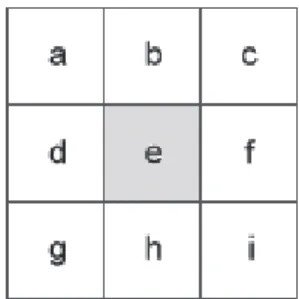
the elevation information of the terrain model by bringing the unit DEM data sequentially. This research conducted a topographic gradient analysis among topographic analysis types. We conducted the terrain slope analysis algorithm based on the difference between the arbitrary elevation point and its adjacent elevation point by using the analysis of continuous Raster data.
As for slope analysis, we adopted the algorithm analyzing the adjacent elevation points and slopes based on the continuous Raster, which is presented to ArcMap, one of the most commonly used methods for topography analysis (Wilson et al., 2007). We calculated the slope by calculating the horizontal and vertical distances of eight elevation points adjacent to the surrounding arbitrary elevation point and calculating the slope of a right triangle.
where column index number
row index number
Denote the Value on level
(2)
deg
×
[
] [
]
×
+g)
×
(3) Here, the terrain surface's
where column index number
row index number
Denote the Value on level
(2)
deg
×
[
] [
]
× +g)
×
is horizontal variation, and
where column index number
row index number
Denote the Value on level
(2)
deg
×
[
] [
]
×
+g)
×
is vertical variation. We used the following algorithm for calculation through eight surrounding elevation points centered on random elevation point.
In case of the above elevation lattices, (Fig. 16) variation in the x-axis direction is,