Comparison of Snow Cover Fraction Functions to Estimate Snow Depth of South Korea from MODIS Imagery

1. Introduction

Accurate data on snow depth are important for coping with heavy snowfall as they help determine

the deployment of individuals and equipment as countermeasures. These data can also be used to calculate the volume of the snowpack, an important consideration for environmental research. There is a

Comparison of Snow Cover Fraction Functions to Estimate Snow Depth of South Korea

from MODIS Imagery

Daeseong Kim*, Hyung-Sup Jung*

and Jeong-Cheol Kim**

*Department of Geoinformatics, University of Seoul

**National Institute of Ecology, Riparian Ecosystem Research Team

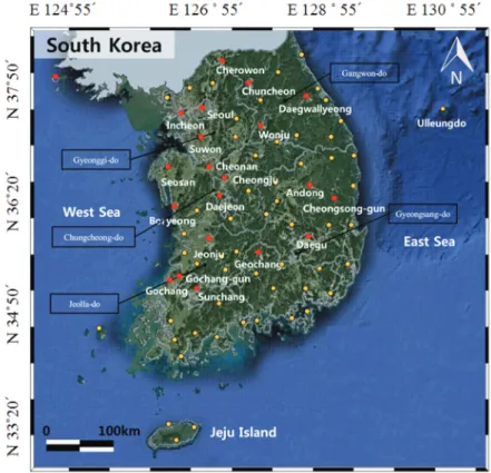
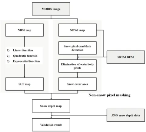
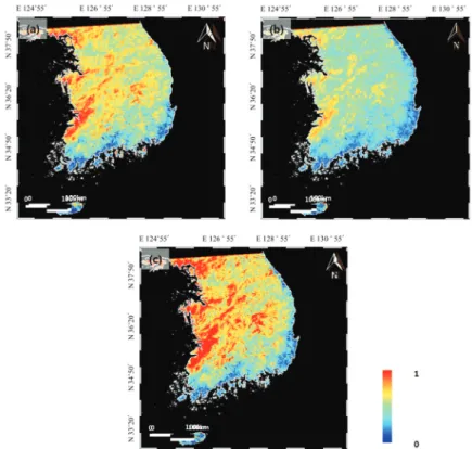
Abstract : Estimation of snow depth using optical image is conducted by using correlation with Snow Cover Fraction (SCF). Various algorithms have been proposed for the estimation of snow cover fraction based on Normalized Difference Snow Index (NDSI). In this study we tested linear, quadratic, and exponential equations for the generation of snow cover fraction maps using data from the Moderate Resolution Imaging Spectroradiometer (MODIS) Aqua satellite in order to evaluate their applicability to the complex terrain of South Korea and to search for improvements to the estimation of snow depth on this landscape. The results were validated by comparison with in-situ snowfall data from weather stations, with Root Mean Square Error (RMSE) calculated as 3.43, 2.37, and 3.99 cm for the linear, quadratic, and exponential approaches, respectively. Although quadratic results showed the best RMSE, this was due to the limitations of the data used in the study; there are few number of in-situ data recorded on the station at the time of image acquisition and even the data is mostly recorded on low snowfall. So, we conclude that linear-based algorithms are better suited for use in South Korea. However, in the case of using the linear equation, the SCF with a negative value can be calculated, so it should be corrected. Since the coefficients of the equation are not optimized for this area, further regression analysis is needed. In addition, if more variables such as Normalized Difference Vegetation Index (NDVI), land cover, etc. are considered, it could be possible that estimation of national-scale snow depth with higher accuracy.

Key Words : snow depth, snow cover fraction (SCF), NDSI (Normalized Difference Snow Index), MODIS, South Korea

Received July 23, 2017; Revised August 14, 2017; Accepted August 17, 2017.

†

Corresponding Author: Hyung-Sup Jung ([email protected])

This is an Open-Access article distributed under the terms of the Creative Commons Attribution Non-Commercial License (http://creativecommons. org/licenses/by-nc/3.0) which permits unrestricted non-commercial use, distribution, and reproduction in any medium, provided the original work is properly cited.

Article

correlation between snowpack and climate change; as the earth becomes warmer, the extent of polar ice and the permanent snow field has shrunk every year. Thus, calculating the amount of snowpack can be used as an indirect method for estimating the pattern and progress of global warming.

Snow depth is also important in water resource management as the winter snowpack is a critical water supply in many countries during seasonal melt.

Accurately calculating the snow water equivalent from the snow pack allows for appropriate water management from this resource. From this perspective, snow depth data is needed at a national scale but an Automatic Weather System (AWS) only provides snow depth at the specific coordinates of its observation stations. Even if snow depth is estimated at a national scale by interpolating the AWS data, the accuracy of these results cannot be guaranteed.

Satellite imagery collects information over large areas as unique pixels, allowing it to overcome the spatial limitations of an AWS and better meet users’

needs. Optical images are particularly advantageous in data acquisition because of their wide swath and short repeat cycle. In order to estimate snow depth using optical satellite imagery, the Snow Cover Fraction (SCF) should be estimated in advance. Barton et al.

(2000) estimated the SCF by using a cubic expression of Normalized Difference Snow Index (NDSI) and Normalized Difference Vegetation Index (NDVI).

Romanov et al. (2003) acquired the SCF by using a simple equation relating the reflectance value of land and snow areas. Salomonson and Appel (2004) used a linear equation for NDSI for calculate SCF; its polynomial regression was derived by using NDSI data from the Moderate-Resolution Imaging Spectroradiometer (MODIS) and Landsat 7 ETM+

images as ground-truth data. Romanov and Tarpley (2007) considered how the relative percentage of deciduous and coniferous forest could affect the estimation of SCF. Lin et al. (2012) fitted the

relationship between NDSI and SCF using an exponential function. Although much research has been conducted on the estimation of SCF from imagery, these studies share a common problem: a limited estimation formula for the study area.

South Korea is a small and mountainous country with highly variable terrain, making it impractical to use the formulas proposed in previous studies.

Therefore, we applied three previously proposed SCF estimation equations (linear, quadratic, and exponential) to South Korea and compared the accuracy of the resulting snow depth images to produce an improved snow depth estimation algorithm for the area

2. Study area and Data

South Korea is a peninsula located between latitudes 33°N and 39°N and longitudes 124°E and 130°E. It experiences four distinct seasons, with winter lasting from the end of November until March of the next year.

Since South Korea is located in a mid-latitude region, is elongated from north to south, and generally has higher terrain in the east than in the west, different snowfall characteristics occur in different regions on the same date. For example, heavy snowfall occurs frequently in eastern mountainous areas such as Gangwon-do, but is uncommon in southern regions such as Gyeongsang-do. Thus a single image may include various geographical features such as mountains and plains along with variable quantities of snow, making South Korea a suitable area for developing snow depth estimation algorithms for use with optical imagery.

In this study, MODIS aqua image obtained on

January 8, 2013 were used and we applied the proposed

equations to a image with the 4th and 7th bands

resampled to 1 km. Band 2 was also used to calculate

the Normalized Difference Water Index (NDWI) value.

The value and 30 m Shuttle Radar Topography Mission (SRTM) DEMs was used to mask waterbodies with high NDSI values. In order to assess the accuracy of each resulting map, we used AWS snow depth data provided by the Korea Meteorological Administration.

In-situ snow depth data which is recorded at 5:00 PM (UTC) was used in order to use the data closest to the acquisition time of the image. All of acquired in-situ data was used except for the Ullengdo with invisible on the image due to the cloud. Table 1 is MODIS channel information used in this study and Fig. 1 shows the study area with the locations of all AWS stations.

3. Method

Fig. 2 shows the overall data-processing flow of this study. First, the extent of snow cover was determined through two stages: snow area detection and waterbody removal. The NDSI value was used to determine the existing snow area and any waterbodies were removed using the DEM and value of NDWI. Next, the snow cover fraction of each pixel was calculated using the NDSI value, generating a different snow cover fraction map with each of the three previously proposed equations. Finally, a snow depth map was calculated from each snow cover fraction map using the formula Fig. 1. Study area and location of Automatic Weather System data used to assess the accuracy of estimated snow depth.

Table 1. Channel information of MODIS used in this study

Channel Wavelength(µm) Resolution(m) Usage

2 0.841 – 0.876 250 NDWI calculation

4 0.545 – 0.565 500 NDSI and NDWI calculation

7 2.105 – 2.155 500 NDSI calculation

proposed by Romanov et al. (2004). We then calculated the root-mean-square error (RMSE) by comparing the calculated values to the actual point data recorded by the AWS stations.

1) Extraction of snow cover area

Classification of snow cover area normally relies on the fact that snow is highly reflective in visible wavelengths but far less so in shortwave infrared (SWIR) wavelengths. The NDSI is generally defined as the ratio of the difference between these two reflectance values. In MODIS Aqua imagery, bands 4 and 6 correspond to visible green and SWIR, respectively, but due to an equipment failure on the satellite, band 6 cannot be used to calculate NDSI.

Therefore, we calculated NDSI with band 7, which is known to have a high correlation with band 6 (Salomonson and Appel, 2006). Therefore, the formula for the calculation of NDSI in this study is as follows:

NDSI = (1)

where ρ

is the reflectance of MODIS Aqua band 4 and ρ

is the reflectance of MODIS Aqua band 7 and it corresponds to visible green and SWIR wavelength., respectively.

Once the NDSI values were generated, the snow cover area was extracted by defining pixels having a value of 0.4 or more as snow candidates. Next, areas of water needed to be removed as their reflectance values can allow for misclassification. We used a NDWI and 30 m SRTM DEM to identify and remove waterbodies from the previously determined snow pixel candidates, producing a final map of snow cover area.

Since the SRTM DEM has only the data of land, it can be used to create a land-masking file. NDWI is a water- sensitive index used to remove shorelines and inland lakes which were not able to removed by using DEM.

ρ

– ρ

ρ

+ ρ

Fig. 2. Flow chart for data processing methods used in this study.

The formula to obtain NDWI is as follows:

NDWI = (2) where ρ

is the reflectance of MODIS Aqua band 2 and corresponds to visible red wavelength.

The reason for using the DEM data is that the NDWI sometimes fails to provide proper masking at the ocean because the value of the pixel value is often wrong.

2) Calculation of SCF

The most important step for snow depth estimation is the calculation of each pixel’s SCF, the percentage of snow-covered area in one pixel. The maximum SCF value occurs between 0 and 1 (0% to 100%). Fig. 3 shows the image that is consisted of four pixels. The blue color means classified pixel to the snow and its area in each pixel represents the SCF of that pixel. That is, SCF of first pixel is 0.53 because the 53% of area is covered with snow in first pixel(Fig. 3(a)). Likewise, SCF of second, third and fourth pixel are 0.09, 0.16 and 0.62, respectively(Fig. 3(b), Fig. 3(b) and Fig. 3(c)).

Although the most accurate approach is visual

analysis using a higher-resolution image, it is not easy to acquire low-resolution and high-resolution images captured in the same region at the same time. Thus SCF is generally calculated indirectly using computable indexes in an image correlated with SCF. Since SCF has a high correlation with NDSI, most studies use NDSI to estimate SCF. Therefore, in this paper, we compared three estimation equations using NDSI values that have shown the most dominant relationship with SCF.

For example, Salomonson et al. (2004) proposed fitting the linear equation with NDSI as follows:

SCF

= a + b*NDSI (3) where a is a constant and b is the coefficient of the first term of the linear equation; this is optimized with values of -0.64 for a and 1.91 for b.

Barton et al. (2000) estimated the relationship between NDSI and SCF using Landsat and MODIS imagery and proposed the estimation of SCF in quadratic form as follows:

SCF

= a + b*NDSI + c*NDSI

(4) ρ

– ρ

ρ

+ ρ

Fig. 3. Demonstration of snow cover fraction as a measure of land area covered by snow.

where a is a constant and b and c are the first and second terms of the quadratic equation; this is optimized with values of 0.18, 0.37, and 0.255 for a, b, and c, respectively.

Lin et al. (2012) fitted NDSI and SCF based on the exponential function as follows:

SCF

= a + b*e

(5) where a, b, and c are the coefficients of the formula;

this is optimized with values of -0.41, 0.571, and 1.068 for a, b, and c, respectively.

3) Calculation of snow depth

The estimation of snow depth in optical imagery is based on a correlation with SCF. As the snow becomes deeper, the reflectivity of the pixel changes, though the change stops after a depth of about 30 cm. Romanov et al. (2003) found that snow depth increases with increasing SCF and that the correlation is similar to the exponential function. From this relationship, they

suggested the following formula:

SD = e

– 1 (6) where a and b are the coefficients of the formula; this is optimized with values of 0.33 and 0 for a and b, respectively.

The snow depth of each pixel was calculated using Equation (5); we then validated the resulting snow depth map by comparing the image with measured values recorded by AWS stations. At this stage, the AWS data was in point format and the snow depth map was represented by pixels with a resolution of 1 km.

Therefore, we validated the accuracy using the interpolated pixel based on the AWS station’s coordinates.

4. Results and Discussion

Fig. 4 shows the images used to mask the non-snow

Fig. 4. Defining snow cover area using satellite imagery: (a) NDSI image of the study area (b) NDWI

image of the study area (c) SRTM DEM of the study area and (d) determined snow cover area.

pixels and the extracted snow cover areas by following in the methods described in section 3a. In the NDSI image, the snow pixel has high value, but it is also calculated to be higher at sea (Fig. 4 (a)). On the other hand, NDWI image shows high values only in the waterbody including the sea. Accordingly, it is possible to prevent the erroneous results by masking a pixel having an NDWI value of 0.1 or more. After this process, some pixels of ocean are not removed due to error of recorded reflectance value at the sensor. So, we used SRTM DEM and it can be effectively remove the that pixels. Finally, the snow cover area is extracted by detecting snow pixel candidates and removing waterbody areas.

Next, SCF maps were generated using the linear, quadratic, and exponential equations described in section 3b (Fig. 5). These confirm that both snow area and waterbody areas have a high SCF value. The linear equation and exponential equation produced results

with similar pattern, but the quadratic equation produced relatively low SCF values and its pattern was different to others. This is due to the difference in the maximum value that can be computed in each equation, about 1.3, 0.8, and 1.25 for the linear, quadratic, and exponential equations, respectively. There is a clear difference in the images as the SCF increases sharply when the NDSI increases steadily in the SCF map generated by exponential equation.

Finally, snow depth maps were produced using the SCF maps as described in section 3c (Fig. 6). Since the snow depth was calculated using the same formula for each map, the differences are more pronounced. The maximum snow depth was calculated to be around 40 cm for the maps based on the linear and exponential equations, but the maximum snow depth was only around 25 cm based on the quadratic equation.

According to the SCF estimation formula, the error range in snow depth results can be up to 15 cm.

Fig. 5. Maps of snow cover fraction (SCF) generated using (a) linear, (b) quadratic, and (c) exponential

equations.

We then graphed the one-to-one correspondence of the snow depth measured by the AWS stations and calculated by the snow depth maps (Fig. 7), with a corresponding RMSE for each equation of 6.73 cm for linear, 5.76 cm for quadratic, and 6.14 cm for exponential. Values plotted above the y=x line represent underestimated snow depth; those below the line represent overestimated snow depth. In the linear case, since the SCF can be calculated as a negative number, there are several cases where the snow depth also has a negative value. In the quadratic case, the snow depth value is generally low because the values were under-estimated at the calculation of SCF stage.

In the exponential case, the data are more tend to be inconsistent than for the other two equations. After examining each point, the most serious mis-matches occurred at the Daegwallyeong, Chuncheon,

Baengnyeongdo, and Daejeon stations. After removing these abnormalities and re-calculating RMSE, the values were reduced to 3.43, 2.37, and 3.99 cm for the linear, quadratic, and exponential equations, respectively.

Commonly the results of snowfall depth tended to be underestimated significantly at the Daegwallyeong, Chuncheon, Baengnyeongdo, and Daejeon AWS stations, where locally-concentrated snowfall may have occurred and the snow in the surrounding urban areas may have been removed. In addition, some AWS are located near pixels including waterbodies, so the influence of surrounding lakes or seas should be considered. In both cases, it is also possible that the pixel values were distorted by fog or thin cloud.

In this study, the proposed SCF estimation equation using NDSI is applied to a single MODIS image and Fig. 6. Maps of snow depth generated using the snow cover fraction calculated from the (a) linear, (b) quadratic,

and (c) exponential equations. Red dots show locations of weather stations used for validation.

three different snow depth maps were generated from the estimated SCF map. Although NDSI has a high correlation with SCF, there are many factors that affect SCF as well as NDSI. In addition, the coefficient of each applied equation is optimized for other test area rather than South Korea. These facts may cause the result to be distorted because it is relatively inaccurate estimation of the SCF for South Korea. In addition, due to the roughness of the MODIS resolution, the result may be distorted if there is pixel that enhances the NDSI such as a local snowfall or lake even though it is not snow. In the case of urban areas, the snow disappears through the snow removal but in-situ points adjacent to the urban area are record the depth of snow;

therefore, the error may occur compared to estimated snow depth. So, the error from this reason should be considered. In fact, the estimated snow depth at four

points with above 10 cm of depth showed significantly difference from the measured value. This may be due to the reasons described above or the result of other complex factors. Nevertheless, in this study, the limitations of each of the three estimation equations were recognized when it was applied for the study area of South Korea. In addition, the ideal formula for South Korea to estimate the depth of snow was proposed and the directions for future research were suggested.

5. conclusion

We applied three previously-proposed SCF equations for the estimation of snow depth from optical imagery to data from South Korea and compared the results as a preliminary step toward developing an algorithm to Fig. 7. Validation results for each snow depth map, comparing actual snow depth with that calculated

from the (a) linear, (b) quadratic, and (c) exponential equations.

estimate the snow depth over this diverse region. The best results were obtained from the quadratic equation, followed by the linear and exponential equations, with RSMEs of. 2.37, 3.43, and 3.99, respectively.

Although the RMSE of the quadratic approach was the best, its under-estimates were too severe to calculate snow depth accurately. In addition, this value likely relates to the small values of the in-situ data constructed in this experiment. In other words, it is highly probable that the RMSE of calculated snow depth from the quadratic approach is the largest when using imagery with a lot of snowfall. Therefore, it is more desirable to design an algorithm using linear-based SCF estimation equations. In order to estimate snow depth with higher accuracy, it is necessary to derive a new estimation formula considering the land type, the humidity content of the snow, and the slope, all of which could affect the SCF estimation. In addition, this study was limited by the use of a single image; better results would be achieved by using a large number of images and uniformly distributed data for snow depth.

By solving these problems first and deriving the best formula for estimating the SCF through regression analysis, future research should be able to develop a snow depth estimation algorithm with higher accuracy for use in the South Korean region.

Acknowledgement

This work was supported by “Development of Scene Analysis & Surface Algorithms” project, funded by ETRI, which is a subproject of “Development of Geostationary Meteorological Satellite Ground Segment (NMSC-2017-01)” program funded by NMSC (National Meteorological Satellite Center) of KMA(Korea Meteorological Administration).

References

Barton, J. S., D. K. Hall, and G. A. Riggs, 2000. Remote sensing of fractional snow cover using Moderate Resolution Imaging Spectroradiometer (MODIS) data, Proc. of the 57th Eastern Snow Conference, Syracuse, New York, USA, May 17-19, pp. 171- 183.

Romanov, P., D. Tarpley, G. Gutman, and T. Carroll, 2003. Mapping and monitoring of the snow cover fraction over North America, Journal of Geophysical Research: Atmospheres, 108(D16).

Romanov, P. and D. Tarpley, 2004. Estimation of snow depth over open prairie environments using GOES imager observations, Hydrological processes, 18(6): 1073-1087.

Romanov, P. and D. Tarpley, 2007. Enhanced algorithm for estimating snow depth from geostationary satellites, Remote sensing of environment, 108(1): 97-110.

Salomonson, V. V. and I. Appel, 2004. Estimating fractional snow cover from MODIS using the normalized difference snow index, Remote sensing of environment, 89(3): 351-360.

Salomonson, V. V. and I. Appel, 2006. Development of the Aqua MODIS NDSI fractional snow cover algorithm and validation results, IEEE Transac - tions on geoscience and remote sensing, 44(7):

1747-1756.

Lin, J., X. Feng, P. Xiao, H. Li, J. Wang, and Y. Li,

2012. Comparison of snow indexes in estimating

snow cover fraction in a mountainous area in

northwestern China, IEEE Geoscience and

Remote Sensing Letters, 9(4): 725-729.