DOI 10.1007/s12303-008-0018-5
Performance of open borehole thermal energy storage system under cyclic flow regime
ABSTRACT: Thermal energy storage can be accomplished through the installation of an array of vertical boreholes. Coupled hydro- geological-thermal simulation of the storage system is essential to provide an optimized configuration of boreholes and operation schedule for the thermal storage system on the site. This paper presents numerical investigations and thermohydraulic evaluation of open borehole thermal energy storage (BTES) system operating under cyclic flow regime. A three-dimensional numerical model for groundwater flow and heat transport is used to determine the annual variation of recovery temperature from the borehole ther- mal energy storage. The model includes the effects of convection and conduction heat transfer, heat loss to the adjacent confining strata, and hydraulic anisotropy. The operation scenario consists of cyclic injection and recovery after holding interval and four periods per year to simulate the seasonal temperature conditions.
For different parameters of the system, performances were com- pared in terms of extraction temperature. The calculated water temperature at the producing pipe remains relatively constant within a certain range through the year. Heat loss, injection/pro- duction rate, and geometrical configuration of boreholes and aqui- fer used in the model are shown to impact the predicted temperature profiles at each stage and the recovery water tem- perature. However, injection temperature and hydraulic anisot- ropy have a less significant effect on the performance of BTES systems. Absolute permeability does not affect the temperature, but is inversely proportional to the injection pressure.
Key words: thermal energy storage, borehole thermal energy storage (BTES), cyclic flow regime, modeling
1. INTRODUCTION
As the demand for energy increases, any work to enhance energy conservation is crucial. Thermal energy storage (TES) system applications around the world have been known to provide economical and environmental solutions to the energy problems (Paksoy et al., 2004). TES systems contribute significantly to improving energy efficiency by providing a buffer to balance fluctuations in energy supply and demand. Ground coupled systems have been receiving attention in recent years because of their energy saving potential and environmental protection when used in TES.
The seasonal variation of temperature in the ground is small relative to the variation in surface air temperature; thus, the ground is normally at a more favorable temperature source
than the air. Therefore, underground thermal energy storage (UTES) is mostly used for seasonal heat/cold storage (Nielsen, 2003). There are several concepts as to how the underground can be used for UTES depending on geolog- ical, hydrogeological, and other site conditions.
One approach for UTES is to install an array of closely spaced vertical boreholes, normally 50–200 m deep. The hole is furnished with pipes for inserting and extracting heat/cold carrying water in the hole. The water is circulated to store or extract thermal energy into or out of the under- ground. This type of thermal storage among UTES systems is called borehole thermal energy storage (BTES) or ducted thermal energy storage (DTES) system utilizing low-tem- perature geothermal resource in the aquifer (Breger et al., 1996; Ohga and Mikoda, 2001; Sanner, 2001; Rafferty, 2003). Depending on the type of application, there are two basic types, open and closed system, being used to transport the heat carrying medium in and out of the holes (Nielsen, 2003). In the open system, which is considered in this study, is the inserting pipe placed with its outlet close to bottom of the hole, whereas the extraction pipe has its inlet opening close to the top of the hole. The water is pumped out of ground and then reinjected into the ground using pipes in the borehole.
The BTES concept requires a much more careful design in order not to risk operational problems such as short-cir- cuiting between the pumping and injection zones (Reffstrup et al., 1994). Recently, the use of numerical simulation has become standard practice in the prediction and evaluation of geothermal performance (Breger et al., 1996; O’Sullivan et al., 2001). In carrying out the design of BTES develop- ment projects, a numerical modeling based on coupled mass and energy transport theory has to be conducted on the behavior of local subsurface geothermal system prefer- ably to study how different aquifer properties and operational conditions are functioning. The results will then guide the decision to specify the design parameters of BTES.
A number of researchers have highlighted the important role of numerical modeling in the analysis of aquifer ther- mal energy storage (ATES) systems (Probert et al., 1994;
Rosen, 1999; Tenma et al., 2003). There appears to be a lack of information regarding the influence of various parame- ters on long-time performance of a BTES system. The present Kun Sang Lee* Department of Environmental Engineering, Kyonggi University, Suwon, Kyonggi-do 443-760, Korea
*Corresponding author: [email protected]
work extends previously reported researches on ATES sys- tems to open BTES systems under various operation param- eters which are key factors influencing long-time performance of BTES systems. The main design considerations involve loading conditions including heat losses, injection/produc- tion temperatures and rates, and configuration of borehole- aquifer system simulating various design and operation sce- narios.
This paper provides coupled hydrogeological-thermal simulation model undertaken to predict the temperature field in the ground. The computer simulation was made for estimation of thermal behavior of ground and recovery tem- peratures from the borehole. Analyses for an open BTES system in a confined aquifer were performed in order to determine how various parameters such as heating and cooling load characteristics, borehole design, and operating systems, affect results of BTES simulations. The evaluation aims to make reliable predictions about future recovery temperatures and temperature distributions in the aquifer given the planned injection/production temperatures and rates.
2. MATHEMATICAL THEORY
To calculate temperatures of the aquifer at different loca- tions, theoretical principles of water flow and heat transfer phenomena are explained.
The continuity of mass for water in association with Darcy’s law is expressed as
(1) where
n: porosity [dimensionless]
ρw: density of water [g/cm3] u: Darcy flux [m/sec]
The water flux from Darcy’s law is
(2) where k [md] is the permeability tensor; μw [cp] the viscos- ity; p [kPa] the pressure; z [m] the vertical depth, and γw [g/
(cm2·sec2)] the specific gravity (= ρwg).
The energy balance equation is derived by assuming that energy is a function of temperature only and energy flux in the aquifer occurs by convection and conduction only. The aquifer is assumed to be continuous and its thermal con- ductivity and volumetric heat capacity are considered to be a function of porosity and the thermal characteristics of water and soil matrix (Nassar et al., 2006). Thermal depen- dence of density, viscosity, thermal conductivity, and heat capacity is not taken into consideration because these parameters vary little in the considered temperature range
of 5-25°C. The resulting general heat balance equation can be formulated as follows;
(3) where,
T: aquifer temperature [°C]
Cvr, Cvw: rock and water heat capacity at constant volume [kJ/(kg·K)]
λT: thermal conductivity of aquifer [W/(m·K)]
qH: enthalpy source per unit bulk volume [kJ/(sec·m3)]
QL: heat loss to overburden and underburden formations [kJ/(sec2·m3)]
The heat transfer with overlying and underlying low-per- meability layers, is assumed to be due solely to thermal dif- fusion and the heat equation is simplified to
(4) where λTe [W/(m·K)] is the thermal conductivity of overbur- den or underburden rock. The heat transfer equation (3), which results from the principle of energy conservation, is coupled with the flow equation from Darcy’s law (2) and the continuity equation (1).
3. MODELING
A proper design of a BTES system under given thermo- hydraulic conditions requires a good understanding of the thermohydraulic processes in the aquifer being the target to use. A multidimensional, finite-difference model for tran- sient subsurface water flow and heat transport is used to solve the complex thermohydraulic problems numerically.
The numerical model includes the effects of hydraulic anisotropy, thermal convection and conduction, and heat loss to the adjacent confining strata. When seasonal storage system is designed, the balance of annual cooling and heat- ing loads plays an important role. In order to decide the sus- tainability of the system for energy storage application, temperatures of producing water should be estimated over a ten-year period.
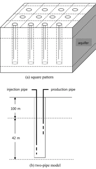
In order to estimate the parameters of an underground system, a general BTES using the open system is consid- ered. A schematic diagram of the system under investiga- tion consisting of the vertical holes drilled in a square pattern and two pipes in each well is shown in Figure 1(a).
The square pattern is simple to drill and connection between drill holes is easy. Water is pumped into the injection pipe at a constant flow rate Q at a temperature Tinj, and the same flow rate of water is recovered from the production pipe. In a large system with repeated patterns, the flow is symmetric
∂t∂
---- nρ( w) ∇ ρ+ ⋅( wu)= 0
u k
μw
---
– (∇p γ– w∇z)
=
∂T∂t
--- 1 n[( – )ρsCvr+nρwCvw] ∇+ ⋅(ρsCvwuT λ– T∇T) qH–QL
=
QL =∇ λ⋅( Te∇T)
around each hole with Q from each pipe confined to the pattern.
A model of two-pipe at the center as shown in Figure 1(b), has been developed to estimate the performance of symmetric array of holes in the square pattern. The outer boundary is represented as a noflow and adiabatic boundary
to simulate symmetry in an array.
Determination of the potential of a specific ground as an effective thermal energy storage medium requires thorough knowledge on the properties of the BTES system. Geolog- ical, hydrogeological and thermodynamic data on the ground, its confining layers and fluid are of importance for simulations. Parameters include porosity and permeability of the storage ground and thermal conductivities and heat capacities of the ground matrix, native groundwater, and confining layers.
Physical and thermal properties of ground considered in the present study are listed in Table 1. The ground and water have constant thermal properties and assumed to be slightly compressible. The volumetric heat capacity and thermal conductivity were identical for the aquifer and the confining layers.
4. RESULTS AND DISCUSSION
To estimate the characteristics of the system, this two- pipe model was run for cyclic flow regime. Heat transfer within the aquifer is simulated by specifying constant tem- perature Tinj at the injection pipe and with the aquifer tem- perature initialized at Ti. An initial storage temperature equal to the ground temperature was assumed, which is taken equal to 20.0°C to start the computations. The fluid and energy flows are calculated for ten years of operation to provide an adequate long-term assessment of thermal storage.
In the cyclic flow regime, water is pumped from one pipe equipped with a pump and reinjected through a second pipe. A complete energy storage cycle is composed of four three-month periods per year to simulate the seasonal con- ditions. Over a finite time period, water at a constant tem- perature Tinj is injected into one pipe at a constant rate, and same amount water is extracted from the other pipe. The thermal field and temperature of produced water, Tprod, are calculated from the numerical solutions of Equation (3) at constant time interval. During the winter, the circulating water collects heat from the earth and carries it into the sur- face. In summer, the system takes heat from surface and Fig. 1. Configuration of BTES system in a square pattern.
Table 1. Hydrogeological and thermal properties of aquifer and water
Aquifer
porosity (n) 0.35
permeability (k) 1,013 md
compressibility of formation (βr) 2.96×10⁻⁶ kPa−1
density of rock (ρr) 2.65 g/cm3
thermal conductivity of rock (λT) 2.88 W/m⋅K
thermal conductivity of overburden/underburden rock (λTe) 2.88 W/m⋅K
heat capacity of rock (Cvr) 0.8864 kJ/kg⋅K
Water
viscosity (μw) 1.1404 cp
compressibility (βw) 4.4×10⁻⁷ kPa−1
density (ρw) 1 g/cm3
heat capacity (Cvw) 4.184 kJ/kg⋅K
places it in the ground. During the rest periods between winter and summer cycles, temperature of a cell containing production pipe is considered as Tprod. Balances between injecting and producing thermal energy and small variation in temperatures are the most desirable case, representing lit- tle fluctuation in extracted thermal energy and sustainable use of aquifer as a BTES system without gradual heating or cooling of the aquifer.
4.1. Heat Loss
Heat transfer from/to overburden and underburden for- mations is considered as an important factor that controls the temperature of produced water. In the present work, results from the heat loss case were compared with those from a case in which heat loss is not included. These for- mations are assumed to have the same thermal properties with aquifer, as stated earlier.
Accounting for the seasonal changes in ground surface temperature, the injected water temperatures were taken as 5°C on the cold side and 25°C on the warm side over three- month periods. During winter and summer cycles, water at a constant temperature is injected into and pumped out from the BTES at a constant rate. Rest periods between 5°C and 25°C water injection periods, neither of injection nor pro- duction was considered.
This model is a unit of the system and composed of two pipes partially-penetrating a confined aquifer of 42 m. As the grid is divided into 17 grid blocks in horizontal direc- tions, and 21 grid blocks in a vertical direction, there are total of 6069 grid blocks. Injection and production pipes are penetrating the aquifer at the intervals of 36-40 m and 2.0- 6.0 m, respectively. The rates of injection or production of 100 m3/day correspond to 0.2354 pore volume of the aqui- fer for three months.
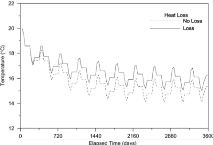
Figure 2 depicts the variation of water temperature in the production pipe. Reflecting the changes in temperature of the injecting water, the recovery temperatures fluctuate with a quarterly year period.
For the case considering heat loss, the recovery temper- atures have been between 15.7°C and 16.9°C during winter after stabilization and decreased slightly with time. The recovery temperature varies roughly between 15.1°C and 16.2°C except the first few years during summer cycle and undergoes a gradual cooling. Due to energy imbalance between the initial temperature of 20°C and average inject- ing temperature of 15°C, the extraction temperature tends to decrease due to a gradual cooling process. Without heat loss, the stabilized temperature at the production pipe fluc- tuates in the fixed ranges of 14.7-15.9°C during winter and 14.1-15.3°C during summer. Temperature is lower than those obtained from the heat loss case and variation is almost same. The results indicate that consideration of the conductive heat exchange with the surrounding rock is nec-
essary in the simulation of BTES.
A study of the recovery temperatures convinced one that thermal breakthrough has not occurred. Relatively small amount of total volume injected during injection cycles indicates that thermal influence between pipes is probably small. The thermal ranges at the recovery pipe imply that the flow conditions of the base case are promising for ther- mal storage. Before examining the influence of a number of parameters on the performance of BTES, the case consid- ering heat loss was considered as a base case for future comparisons in the present simulations.
4.2. Injection Temperature
To demonstrate the effect of temperature difference on long-time thermal storage performance, additional simula- tions were performed using different combinations of water temperature at the injection side. Having average value of 15°C, the water temperature was constant during each three-month injection period and had values of 1°C/29° and 9°C/21°C, respectively. Other conditions and parameters were not changed from the operation scenario of the base case.
Variation of water temperature is obtained using the model is given in Figure 3 for different injection tempera- tures. The stabilized recovery temperature is changed from 15.9-16.5°C to 15.6-17.2°C during winter and from 15.4- 16.0°C to 14.7-16.2°C during summer by increasing the temperature difference around the year at the injection pipe from 12°C to 28°C. Increased range in extraction temper- atures was obtained with increasing differences in injection temperature. The range of variation of case 1°C/29°C is the highest and 2.50-2.67 times higher than that of 9°C/21°C which is the smallest. Simple calculations of temperature ranges imply that injection temperatures considerably affect the results.
Fig. 2. History of calculated temperatures of produced water obtained from simulations with different heat loss conditions.
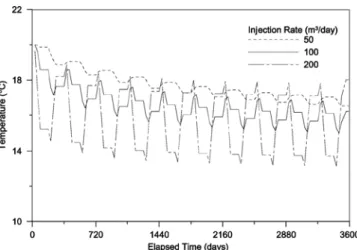
4.3. Flow Rate
The aim of this simulation is to study how different injec- tion or production flow rates affect the recovery of thermal energy from the borehole. The calculations were performed for borehole and aquifer configuration which is the same as the base case. However, in this simulation, the flow rates are changed to 50, 100, and 200 m3/day. These rates are equivalent to injecting 0.1177, 0.2354, and 0.4708 pore vol- umes for a three-month period.
Figure 4 presents variation of recovery temperature for three different flow rates. It was observed that the higher flow rate for a given BTES gives the larger variation in recov- ery temperature. This result comes from relatively large flow rates compared with the pore volume of the aquifer avail- able for thermal storage. Increasing the flow rate four times yields recovery temperature changes from 16.8-17.2°C to 13.7-17.8°C during winter and from 16.6-17.2°C to 13.7- 17.1°C during summer, which mean increases in the ranges
of stabilized temperature from 0.4°C to 4.1°C during winter cycle and from 0.6°C to 3.4°C during summer cycle.
Increasing the flow rate four times results in increases in the ranges of temperature by 10.3 times during winter cycle and 5.7 times during summer cycle. The result suggests that, everything else being the same, the use of less flow rate is a promising flow condition due to small net change in recovery temperature. However, decreasing the flow rate considerably less than an appropriate value would not be effective because the resulting decrease in the amount of available thermal energy would be a problem.
4.4. Areal Extent
Selection of storage size is very important for BTES sys- tem. One objective with the numerical simulations is to find the ground-borehole configuration to make the energy stor- age as dense as possible. In attempts to investigate effects of areal extent, pumping and injection were simulated for three cases considered, 39 m × 39 m, 51 m × 51 m, and 63 m
× 63 m, which correspond to the interwell distances between neighboring wells of 39 m, 51 m, and 63 m, respectively.
Aquifer thickness remains same with the base case. These distances correspond to 0.4025, 0.2354, and 0.1543 pore volume of the aquifer for three months of injection or pro- duction at 100 m3/day.
Long-time variation of water temperature from storage is illustrated in Figure 5 for different storage volumes to deter- mine an optimum tank size. It illustrates a larger extent or larger borehole spacing delays cooling process in thermal storage substantially and results in higher recovery temper- ature. By increasing the pore volume of the aquifer by 2.6 times, it does not significantly improve the performance of BTES systems. The ranges of stabilized recovery temper- atures decrease from 15.5°C-16.7°C to 16.2°C-17.3°C during winter and from 14.4°C-15.6°C to 15.6°C-16.7°C during summer.
Fig. 3. History of calculated temperatures of produced water obtained from simulations with different injection temperatures.
Fig. 4. History of calculated temperatures of produced water obtained from simulations with different injection/production flow
rates. Fig. 5. History of calculated temperatures of produced water
obtained from simulations with different areal extents.
4.5. Screen Location
To investigate the influence of the screen location in the performance of BTES system, injection pipes with screen at 14-18 m, 24-28 m, and 36-40 m were considered. Screen of the production pipe is installed at 2-6 m for all cases.
Figure 6 shows that lowering the injection pipe or increasing the interval between pipes results in a significant drop in the range of temperature. The range of average sta- bilized recovery temperature is changed from 10.5-21.0°C to 15.7-16.9°C during winter and from 10.5-21.0°C to 15.1- 16.2°C during summer by increasing screen distance. The temperature variation is improved to 10% when distance between screens was changed from 12 m to 24 m. The results demonstrate the importance of aquifer thickness which determines the screen distance. Larger variations for shorter screen-to- screen distance result from the fact that the thermal front of injected water approaches the produc- tion pipe within each operation period. Therefore, the region near a producing pipe is considerably affected by injected water. This observation emphasizes the importance of ensuring that adequate vertical distance between injec- tion and production pipes is used, taking into account the thermal and hydraulic transport of injected water. The ground height can be a limitation of potential for imple- menting BTES.
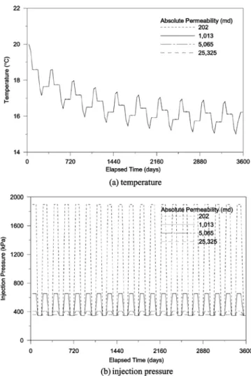
4.6. Absolute Permeability
To examine the effect of absolute permeability of the aquifer the thermal storage performance, additional simu- lations were performed. All other conditions are same to the base case except for considering permeabilities of 202 md, 1,013 md, 5,065 md, and 25,325 md.
Long-time variation of water temperature presented in Figure 7(a) illustrates little difference between results. This observation results from the fact that the flow rates of
injected and produced water are same for all cases and have no effect on the temperature of produced water. However, the injection pressure is inversely proportional to the abso- lute permeability. As indicated in Figure 7(b), the injection pressure for low permeability aquifer is almost five times higher than that of base case. Everything else being the same, the effects of absolute permeability on the injection would be substantial, even though being negligible on the temperature of produced water.
4.7. Permeability Anisotropy
The permeability in horizontal direction can be signifi- cantly greater than that in vertical direction. In this simulation, the effect of permeability anisotropy on the performance of a BTES system was examined. All other conditions are similar to the base case except for considering anisotropy in permeability by replacing vertical permeability with differ- ent values. Permeabilities in x and y directions are kept con- stant. The ratios of vertical to horizontal permeability Fig. 6. History of calculated temperatures of produced water
obtained from simulations with different screen locations.
Fig. 7. History of calculated temperatures of produced water and injection pressure obtained from simulations with different abso- lute permeability.
considered in this study are 1.0, 0.5, and 0.1.
Water temperature from the storage tank is demonstrated in Figure 8 for three different permeability ratios. A strong dependence is observed between the performance of BTES systems and the permeability anisotropy. The temperature values for kz/kx= 1.0 show the largest variation, while those of kz/kx= 0.1 show little variation during recovery. The increases in the range of extraction temperatures are about 3.7 times during winter and 2.8 times during summer over the stabilized period. This observation can be explained by the fact that the injected water have a minimal effect on the region near a producing pipe due to less vertical flow of injected water is for a highly anisotropic case. Everything else being the same, the effects of permeability anisotropy would be significant.
5. CONCLUSIONS
A numerical simulation model for designing and evalu- ating BTES was developed to evaluate the effects of the design parameters. The results of long-time thermal behav- ior of an open BTES system under cyclic operation meth- ods were examined. The effects of various operating conditions and aquifer characteristics on computed values of producing temperature were studied for a 10-year con- tinuous injection and production. The numerical calcula- tions on the hypothetical two-pipe system demonstrated that this simulation has great potential in evaluating the temper- ature field and the recovery temperature of BTES and deter-
mining the most efficient system operation.
The thermal behavior of the storage system is shown to depend on various operational and geometrical parameters including operation schedules, injection temperature, injec- tion/production rates, geometrical configuration of borehole and aquifer, and permeability that impact the predicted recovery water temperature. Among them, injection rate and aquifer thickness are extremely important on the per- formance of BTES systems. Small variations in injection temperatures, low flow rate, and large surface to volume ratio are recommended as an effective BTES because of small loss and little fluctuation in extracted thermal energy.
REFERENCES
Breger, D.B., Hubbell, J.E., Hasnaoui, H.E., and Sunderland, J.E., 1996, Thermal energy storage in the ground: comparative anal- ysis of heat transfer modeling using U-tubes and boreholes. Solar Energy, 56, 493−503.
Nassar, Y., ElNoaman, A., Abutaima, A., Yousif, S., and Salem, A., 2006, Evaluation of the underground soil thermal storage prop- erties in Libya. Renewable Energy, 31, 593−598.
Nielsen, K., 2003, Thermal energy storage. A state-of-the-art, NTNU, Trondheim.
Ohga, H. and Mikoda, K., 2001, Energy performance of borehole thermal energy systems. Proc. of Seventh International IBPSA Conference, p. 1009−1016.
O’Sullivan, M.J., K. Pruess, and Lippmann, M.J., 2001, State of the art of geothermal reservoir simulation. Geothermics, 30, 395−429.
Paksoy, H.O., Gurbuz, Z., Turgut, B., Dikici, D., and Evliya, H., 2004, Aquifer thermal storage (ATES) for air-conditioning of supermarket in Turkey. Renewable Energy, 29, 1991−1996.
Probert T., Hellsröm, G., and Glaesson, J., 1994, Thermohydraulic evaluation of two ATES projects in southern Sweden. Proc. of Int’l Symp. on Aquifer Thermal Energy Storage, p. 73−81.
Rafferty, K., 2003, Ground water issues in geothermal heat pump systems. Groundwater, 41, 408−410.
Reffstrup, J., Sørensen, S.N., and Qvale, B., 1994, Design and system integration of groundwater heating and cooling plants. Proc. of Int’l Symp. on Aquifer Thermal Energy Storage, p. 15−28.
Rosen, M.A., 1999, Second-law analysis of aquifer thermal energy storage systems. Energy, 24, 167−182.
Sanner, B., 2001, Shallow geothermal energy. GHC Bulletin, 19−25.
Tenma, N., K. Yasukawa, and Zyvoloski, G., 2003, Model study of thermal storage system by FEHM code. Geothermics, 32, 603− 607.
Manuscript received September 20, 2007 Manuscript accepted May 30, 2008 Fig. 8. History of calculated temperatures of produced water
obtained from simulations with different permeability anisotropy.