This is an Open Access article distributed under the terms of the Creative Commons Attribution Non-Commercial License (http://creativecommons.org/licenses/
Statistical notes for clinical researchers:
A one-way repeated measures ANOVA for data with repeated observations
http://dx.doi.org/10.5395/rde.2015.40.1.91
Repeated measures and correlated data
Repeated measurements can be obtained in many situations. A simple example is a pre-post design to assess the intervention effect. With respect to conditions, e.g., treatment A, B, and C, different treatments may be applied to the same group of subjects repeatedly according to the designated time schedule to compare the effects of treatments. In perspective of time, we may measure children’s height repeatedly to know the growth pattern. In the field of dentistry, we measure the periodontal pocket depths of a tooth repeatedly at different surfaces: buccal, lingual, mesial, and distal. Common characteristics of these repeated measurements include correlations of the data points obtained by the same object, person, tooth, etc. The paired t-test is an analyzing method of correlated samples with two time points or occasions. For three or more time points or repeated conditions, we may use the repeated measures ANOVA which is equivalent to the one-way ANOVA for independent samples. Therefore, continuous outcome variables and categorical independent variables are the basic requirements.
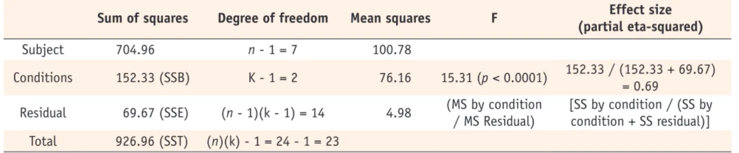
Comparison of one-way repeated measures ANOVA and classical one-way ANOVA Table 1 shows a hypothetical data with repeated observations, P1, P2, and P3, which may represent scores measured in different conditions or different time points. If we disregard the correlated structure of three scores, the data can be analyzed using the one-way ANOVA. The classical one-way ANOVA decomposes the total variation of scores (SST, total sum of squares) into between-group variance (SSB, SS by conditions in Table 2) and within-group variance (SSW, SS residual in Table 2). The total variation is explained by SSB of different conditions (P1, P2, and P3), and the remainder is a substantial amount of unexplained within-group variance (Table 2). On the other hand, in the one-way repeated measures ANOVA, SSW is divided into SS by subject and unexplained SS (SSE, error sum of squares), which results in a significant difference among different conditions after considering subject effects, as shown in Table 3.
In the classical ANOVA, different conditions do not make significant differences (p = 0.1503), while the repeated measures ANOVA obtain significant differences (p < 0.0001).
The variance proportion explained in ANOVA is used as an ‘effect size’ which represents the degree how the analysis is effective in explaining the variance of outcome variable.
In result of the repeated measures ANOVA, ‘the partial eta squared’ is calculated by dividing the variance explained with the condition (SS by condition) by the total variance (SS by condition +SS residual), excluding variance by subjects. In Table 3, the partial eta squared is calculated as 0.69.
Hae-Young Kim
Department of Dental Laboratory Science and Engineering, College of Health Science & Department of Public Health Science, Graduate School, Korea University, Seoul, Korea
*Correspondence to Hae-Young Kim, DDS, PhD.
Associate Professor, Department of Dental Laboratory Science &
Engineering, Korea University College of Health Science, San 1 Jeongneung 3-dong, Seongbuk-gu, Seoul, Korea 136-703
TEL, +82-2-940-2845; FAX, +82-2- 909-3502, E-mail, kimhaey@korea.
ac.kr
Kim HY
Multivariate and univariate tests
The multivariate tests analyze multiple variables (P1, P2, P3) as one observation using a ‘wide-form’ data that one person has one record with P1 to P3. The multivariate approach requires a sufficient number of subjects (e.g., larger than 30) as the number of person is the number of information. Also a record with any missing value is deleted, therefore even small number of missing values may lead to substantial loss of information. When sample size is large, Pillai’s trace and Wilk’s lambda have similar power and show similar results (Please refer [g] of SPSS analysis results).1 The univariate tests are analyzing ‘long form’ data that one person has multiple records by occasions, e.g., three records per person in this example.
The univariate tests have more power based on the increased number of information and have relative advantage in treating missing values that only the missing occasions are deleted. In case with many missing values, only the univariate approach works. However additional assumption, ‘sphericity’ is enquired to obtain reasonable analysis results by the univariate tests.
Table 1. Hypothetical data with repeated observations
Condition Difference
Subject P1 P2 P3 Subject mean P2-P1 P3-P1 P3-P2
1 24 29 36 29.7 5 12 7
2 31 35 39 35.0 4 8 4
3 20 15 20 18.3 -5 0 5
4 17 21 24 20.7 4 7 3
5 22 22 25 23.0 0 3 3
6 25 30 35 30.0 5 10 5
7 27 27 30 28.0 0 3 3
8 19 20 24 21.0 1 5 4
Mean 23.1 24.9 29.1
Grand Mean 25.7
Variance 11.9 16.0 1.9
Table 2. Summary table for the classical on-way ANOVA (incorrect)
Sum of squares Degree of freedom Mean squares F Effect size (eta squared) Conditions 152.33 (SSB) k - 1 = 2 76.16 2.06 (p = 0.1503) 152.33 / 926.96 = 0.16
Residual 774.63 (SSW) (n - 1)(k) = 21 36.89 (MS by condition
/ MS Residual) (SS by condition / SST) Total 926.96 (SST) (n)(k) - 1 = 24 - 1 = 23
Table 3. Summary table for the one-way repeated measures ANOVA
Sum of squares Degree of freedom Mean squares F Effect size (partial eta-squared)
Subject 704.96 n - 1 = 7 100.78
Conditions 152.33 (SSB) K - 1 = 2 76.16 15.31 (p < 0.0001) 152.33 / (152.33 + 69.67)
= 0.69 Residual 69.67 (SSE) (n - 1)(k - 1) = 14 4.98 (MS by condition
/ MS Residual) [SS by condition / (SS by condition + SS residual)]
Total 926.96 (SST) (n)(k) - 1 = 24 - 1 = 23
The univariate tests assume an equal correlation between the repeated measures which is called ‘sphericity’ condition.
Sphericity refers to the condition where the variances of the differences between all possible pairs of groups (i.e., levels of the independent variable, ‘conditions’ here) are equal. Table 3 is the result based on the sphericity assumption. However, variances in differences between pairs of conditions, P2-P1, P3-P1, and P3-P2 are 11.9, 16.0, and 1.9, respectively, which seem fairly different (shown in the right side of Table 1). The Mauchly’s test which evaluates the sphericity condition showed that the assumption of sphericity was unsatisfied (p = 0.025, [h] of SPSS results), thus additional remedy steps should be taken. The remedy is to adjust degrees of freedom of numerator and denominator by multiplying the adjustment factor, ε (epsilon). Two kinds of epsilon, Greenhouse-Geisser and Huynh-Feldt epsilon ([h] of SPSS results) are applied to the test of within-subject effect ([i] of SPSS results). If the epsilon is close to one, which means the sphericity assumption is met, then there is no need of adjustment. The guideline of epsilon is determined by the Greenhouse-Geisser epsilon, 0.75;
if larger than 0.75 then apply the Huynh-Feldt epsilon, otherwise, apply the Greenhouse-Geisser epsilon.2 In this example as the Greenhouse-Geisser epsilon was 0.586, we interpret the corrected results in (i) of the SPSS results by applying epsilon to degrees of freedom of ‘repeat 1’ and error portion (p = 0.003) with the heading Greenhouse-Geisser. The pairwise comparison of main effects of P1, P2, and P3 shows that significant differences are found in P3 and other two occasions by applying the Bonferroni correction which controls the type one error rate ([k] of SPSS results). We could see that mean of P3 is significantly different from those of P1 (p = 0.011) and P2 (p < 0.001), while means of P1 and P2 are similar (p = 0.585) as shown in table (k) of SPSS output.
Other outputs
Assessment polynomial terms show that assuming linear relationship among repeated measurements is appropriate ([j] of SPSS results). Also the Profile plot ([l] of SPSS results) provides the trend of the repeated measurements. Tests of between- subjects effects traditionally provided by the repeated measures ANOVA SPSS output (not shown) represent the comparison of simple averaged values among groups without accounting for correlated structures; therefore the importance of the result is little in respect to the analysis of correlated data.
The procedure of the one-way repeated measures ANOVA using SPSS statistical package (SPSS Inc., Chicago, IL, USA):
(a) Data (b) Analyze-General Linear Model -
Repeated measures (c) Factor name (repeated measure) and number of levels (3) - Define
Kim HY
(d) Define repeated variables (e) Request plots (f) Compare main effect - Bonferroni method
(g) Result of multivariate tests
(h) Test of sphericity
(i) Tests of within-subjects effects
References
1. Park E, Cho M, Ki CS. Correct use of repeated measures analysis of variance. Korean J Lab Med 2009;29:1-9.
2. Field A. Repeated measures designs: discovering statistics using SPSS. 3rd ed. London: SAGE Publications Ltd; 2009.
Chapter 13.
(k) Pairwise comparison
(l) Profile plots
30
28
26
24
Estimated marginal means of MEASURE_1
1 2 3 Repeat 1
Estimated marginal means