Effectiveness of an Exponentially Smoothed Ordering Policy as Compared with Kanban System
Takayoshi Tamura
1†․Tej S. Dhakar
2․Katsuhisa Ohno
3*1
Nagoya Institute of Technology, Gokiso-cho, Syowa-ku, Nagoya 466-8555, Japan
2
Southern New Hampshire University, 2500 North River Road, Manchester, NH 03106, USA
3
Aichi Institute of Technology, 1247 Yachigusa, Yakusa-cho, Toyota 470-0392, Japan
The Kanban system in Just-In-Time (JIT) production is very effective in reducing the inventories when con- sumption rate of the final product is relatively stable. When large fluctuations exist in the consumption rate, a new production ordering policy in which the production order quantity is determined by smoothing the demands exponentially is more suitable. This new ordering policy has not been investigated sufficiently. In this research, a multi-stage production and inventory system with stock points for materials and finished items located at each stage is considered. Approximations of average inventories at each stage in the system are derived theoretically.
Numerical simulations are carried out to assess the accuracy of approximations and to evaluate the effectiveness of the new ordering policy as compared with the Kanban system. As a result, it is shown that the new ordering policy can achieve significantly lower inventory costs than the original Kanban system. The new ordering policy thus emerges as a key concept for an effective supply chain management.
Keywords: Multi-stage Production and Inventory System, Production Ordering Policy, Exponential Smoothing,
Kanban, Jit, Supply Chain Management
1. Introduction
A typical tool for controlling production and pro- curement in the JIT system is the “Kanban”
(Monden 1998). Many articles exist dealing with the performance of the Kanban system, e.g., Krajewski
et al., 1987, Miltenburg 1997 and Spearman et al.,1990. In order to make the production and procure- ment more efficient using the Kanban system, the consumption rate of a part used for production is leveled at the final assembly line in the automobile industry (Monden 1998, Korkmazel et al., 2001 and Kubiak 1993). In practice, however, the number of kanbans removed according to part consumption in a time period fluctuates.
Kotani (1990) who worked as a middle manager at Toyota Motor Co. proposed a new production ordering policy in which the production order quan- tity in each period is determined by smoothing demands. However, he does not discuss how his policy is effective in reducing the total inventory.
We call Kotani’s concept “exponentially leveled or- dering policy” (referred to as EXPLEVEL here- after). So far, this ordering policy has been inves- tigated in a very few papers (see Tamura et al., 2005, 2006). In Tamura et al. (2005) the effective- ness of the EXPLEVEL system is discussed for a single stage model as compared with Kanban and CONWIP by Spearman et al. (1990).
In this research, we derive approximations of aver- age inventory at each stage in a multi-stage pro-
Authors would like to acknowledge Professor Ilkyeong Moon, Pusan National University, and Korean Institute of Industrial Engineers for giving us the opportunity to contribute this article to the Journal.
†Corresponding author : Takayoshi Tamura, Nagoya Institute of Technology, Gokiso-cho, Syowa-ku, Nagoya 466-8555, Japan Tel : +81-52-735-5390, E-mail : [email protected]
Received December 2007; revision received january 2008; accepted january 2008.
duction and inventory system when an exponentially smoothed ordering policy is used to determine pro- duction order quantities. Using derived approximations together with simulation experiments, the effective- ness of the exponentially smoothed ordering policy is then compared with the original Kanban system.
The paper is organized as follows. Section 2 lists the assumptions and notation used in formulating the mathematical models. In section 3, we formulate the mathematical models for the original Kanban system and the EXPLEVEL system. In section 4, we derive approximations for variance and expect- ation of inventories at each stage when the pro- duction quantity is smoothed at the final stage. In section 5, we evaluate quantitatively the perform- ance of the EXPLEVEL system as compared with the Kanban system using simulation experiments together with derived approximations for a three- stage production and inventory system. We also briefly discuss the application of the EXPLEVEL system to supply chain management. Section 6 con- cludes the paper.
2. Model Assumptions and Notation
The following assumptions are made for modeling the Kanban and EXPLEVEL systems:
(1) A single item is produced at each stage.
(2) Two stock points, one for materials and the other for the finished item, exist at each stage.
(3) The production capacity at each stage is unlimited.
(4) Product demand at the final stage follows an identical independent distribution during each period.
(5) Pro duct demand during each period is ship- ped to the customer at the end of the period, if inventory is available.
(6) Finished item at a stage is shipped to the successor stage at the end of each period.
(7) Production order at each stage is placed at the beginning of each period, while the ma- terial replenishment order at each stage is placed at the end of each period.
(8) Material needed for production during a peri- od is required at the beginning of the period for each stage.
(9) Replenishment order quantity for material at
the end of each period is equal to quantity of the material consumed for production dur- ing the period for each stage.
(10) Three types of lead-times are considered, which are production lead-time, lead-time to send replenishment order to the predecessor stage and shipment lead-time for conveying the finished item to the successor stage.
They are known and constant.
(11) Shipment backlog of finished item from each stage to the successor stage is allowed.
(12) To produce one unit of item at each stage requires one unit of material.
(13) Kanban container size is set to one.
(14) No defectives are produced.
Notation is defined as follows:
: The number of stages,
: Stage index,
: Demand for the final product in period
,
: Production lead-time at stage
, where
≥
,
: Lead-time to send replenishment order from stage
to stage
, where
is a giv- en non-negative integer,
: Shipment lead-time to send finished item from stage
to stage
, where
is a given non-negative integer,
: Replenishment lead-time for materials used at stage
, where
is re- plenishment lead-time for the raw material required at stage 1,
: Production order quantity at stage
in period
,
: Production quantity realized under consid- eration of material constraint at stage
in period
,
: Material replenishment order quantity at stage
at the end of period
,
: Shipment quantity of finished item sent from stage
to stage
at the end of period
,
: Inventory of finished item at stage
at the beginning of period
, where
is final product inventory at the final stage,
: Inventory of finished item at stage
at the end of period
,
: Shipment backlog of finished item to be
sent from stage
to stage
in peri-
od
, which is caused by a shortage of
Stage 1
Product inventory Raw Material
inventory Supplier
Material flow Information flow
S2,t Stage
2
Inventory
X2,t-a2 X2,t
S1,t - e1-1 X1,t-a1
X1,t y1,t-b1-1
y1,t = x1,t O1,t = S1,t-1 Y2,t = X2,t O2,t = S2,t -1 Dt
d2 e1
Figure 1. Two-stage production system managed by Kanban
Stage 1
Stage 2
Y1,t = X1,t O1,t Y2,t = X2,t O2,t Dt
Product inventory Raw Material
inventory Supplier
Material flow Information flow Inventory
y1,t - b1-1
d2
e2
X1,t X1,t - a1 S1,t - e1-1 X2,t X2,t - a2 S2,t
β1 β2
Figure 2. Two-stage production system managed by EXPLEVEL system
finished item at stage
, where
is
product shipment backlog for customers,
: Production backlog at stage
in period
, which is caused by a shortage of material used for production at stage
,
: Material inventory at stage
at the be- ginning of period
,
: Material inventory at stage
at the end of period
,
: Safety factor for allowable stock-out pro- bability
with respect to finished item at stage
,
: Safety factor for allowable stock-out pro- bability
with respect to material used at stage
,
: Exponential smoothing factor used for smoo- thing production quantity at stage
,
≤
: Production backlog caused by production smoothing at stage
,
: Variance of random number,
: Expectation of random number
, and
: Smallest integer which is larger than or equal to
.
3. Model Description
3.1 Production and Inventory Model
Based on the assumptions stated in section 2, the production and inventory model can be formulated as follows:
(1) Production quantity realized under consid- eration of both available material and pro- duction order quantity:
+
for
⋯(1) (2) Production backlog at stage
:
for
⋯(2)
(3) Finished item inventory at stage
at the be- ginning of period
:
for
⋯(3) (4) Material inventory at stage
at the begin-
ning of period
:
for
⋯(4) Note that the difference between subscripts
in (3) and
in (4) is because the pro- duction order is released at the beginning of each period while shipment is made at the end of each period.
(5) Material replenishment order quantity which is ordered at the end of each period (see Assumption 9) is given by the following equation:
for
⋯(5)
(6) Shipment quantity of item sent from stage
:
=
⋯
Note that equation (6) allows us to receive a re- plenishment order from the successor with zero lead-time when
.
(7) Backlog of shipment quantity to be sent from stage
to the next stage:
⋯
(8) Finished item and material inventories at
stage
at the end of period
:
⋯
(8)
⋯
(9)
3.2 Production Order Quantity 3.2.1 Kanban system
<Figure 1> depicts the operation of the Kanban system. In the Kanban system, production order quantity at a period is simply set to the quantity of finished item consumed during the last period, i.e.
⋯
(10)
3.2.2 EXPLEVEL system
<Figure 2> depicts the operation of the EXPL- EVEL system consisting of two stages. In this sys- tem, the production order quantity is determined by smoothing demands from the next stage exponen- tially.
For the material at each stage, it is assumed that the replenishment order quantity is set equal to the quantity consumed for production at the stage in each period. Based on the assumption, the EXPLEVEL system can be modeled as follows:
(1) Production order quantity at stage
:
for
⋯(11) As shown in section 4.1, the production order quantity given by (11) is identical to the quantity obtained by smoothing demands from the next stage exponentially if the production order quantity is not restricted to integer value. Note that the concept of production smoothing in (11) is different from the production smoothing in a mixed-model line ach- ieved by the traditional goal chasing method.
(2) Backlogs caused by production smoothing:
for
⋯(12)
4. Approximations for EXPECTATION and Variance of Inventories
4.1 Variance of Inventory in EXPLEVEL System
In the EXPLEVEL system, the demands are ex-
ponentially smoothed to determine the production
order quantity at each stage as given by (11). By
ignoring any shortage of product and material as well as ignoring the integer condition for the order quantity, the production quantity (11) at the final stage is approximated by substituting (12) as fol- lows:
≅
= ≅
(13) The last result was given by Kotani (1990) and Tamura et al. (2005). This is the reason why the ordering policy is called “exponentially leveled or- dering policy”. Equation (13) can be expressed by
≅ ≅
≥
(14) In the following discussion, we assume that the production order smoothing is performed only at the final stage and the other stages utilize the Kanban rule to determine their order quantities.
Consider expectation and variance of inventories at the final stage. For the final stage, if we assume that the shortages for product and material are small enough to be ignored, for the final stage the shipment quantity given in (6) is approximated by demand, i.e.
≅
By substituting this approximation and equations (3) and (14) into (8),
≅
≅
≥
≥
≅
≥
≥
≥
≅
≥
≥
≥
is obtained. If we apply the following relation for any
, where
, to the last equation.
(15)
then we obtain the following approximation:
≅
≥
(16) Since the demand is assumed to be i.i.d., the variance of the right hand side in (16) (denoted by
) is given by
(17)
where
Var[
]. The
can be used as an approximation for the variance of
for the EXPLEVEL (denoted by Var[
]), i.e.
Var
≅ For the material at the final stage, when the ma- terial replenishment is performed by the JIT rule, the following approximation holds.
≅
≅
(18)
Substituting (14) into (18), we obtain
≅
≅
≥
Since demand is assumed as being i.i.d., applying (15) the variance of the last equation (denoted by
) is given by
(19)
And then the variance of
denoted by Var [
] is approximated by
Var[
]
≅ Using the Kanban rule to determine production quantity and material replenishment quantity at each stage
⋯ , variances of inven- tories at stage
can be derived in a manner sim- ilar to the derivation of (19) assuming that the shor- tages of finished item and material are small en- ough to be ignored. The results are given below:
for
⋯ (20)
for
⋯ (21) where
and
are the ap- proximated variances for product and material in- ventories, respectively, at stage
at the end of period when the smoothing factor at the final stage
is given.
Let E[
] denote the expectation of random variable
for each
. Using (17), (20) and (21), the following approximations for expectation and variance of product and material inventories in EXPLEVEL can be obtained, where notation
and
are safety factors for allowable stock-out rates
of product and
of material, respectively, at stage
:
Var
≅ for
⋯(22)
for
⋯(23) E
≅ for
⋯(24) E
≅ ,
for
⋯(25) Var
≅ for
⋯(26)
for
⋯ (27) E
≅ for
⋯ (28) E
≅ for
⋯ (29) In order to derive (17), (20) and (22), the mutual interaction between material shortage and pro- duction delay are not taken into consideration. For instance, (17) does not consider any shortage of material and hence an actual stock-out rate of final product will become larger than
due to short- age of material. Conversely (21) will overestimate the safety stock level of the material. In order to obtain tighter approximations, both
and
in (23) and (27) will be revised by simu- lation experiments (Tamura et al., 2005).
4.2 Expectation of Inventory in Kanban System
When the smoothing factor
is equal to one, the EXPLEVEL system becomes equivalent to the Kanban system. Substituting
= 1, (17) and (20) are simplified to
≅
for
⋯ (30) and (21) is also simplified to
≅
for
⋯ (31) Substituting (30) and (31) into equations from (22) to (29), we obtain formulas for variance and expectation of product inventory as well as materi- al inventory for the Kanban system.
4.3 Delay due to Production Smoothing
Ignoring any shortage of product and material as well as ignoring the integer condition for the order quantity, since
and
are approximately equal to
and
, respectively, (11) and (12) at the final stage can be approximated by
≅
≅
Substituting the first of these two equations given above into the second, we obtain
≅
Then taking the expectation of both sides in the above equation leads to the following equation:
E
≅
(32)
5. Numerical Experiments
This section discusses the accuracy of approxima- tions derived in the previous section and the effec- tiveness of smoothing the production quantity at the final stage in the EXPLEVEL system as com- pared with the Kanban system.
5.1 Parameters and Conditions for the Simulation
The following parameters were used in the simu- lation experiments:
(1) Number of stages : The production system con- sists of three stages, i.e.,
.
(2) Demand : Binomial distribution is used, which is defined by two parameters (say,
and
) and the expectation and variance are given by
and
(1-
) respectively. For the ex- periments, we assume that
= 0.5 and
= 30 or
= 100. Then E [
] = 15,
= 7.5 for
= 30 and E [
] = 50,
= 25 for
= 100.
(3) Lead-times : Production lead-time, replenish- ment order sending lead-time and shipment lead-time are set as follows:
= 3,
=
= 2,
= 5,
=
= 2,
=
+
= 4,
= 2,
= 1,
=
= +
= 3
(4) Stock-out rate : We assume
=
= 5% for all
= 1, 2, 3 and then safety factor for each stage
= 1, 2, 3 is set to
=
= 1.645
which is obtained from the standard normal dis- tribution.
(5) Exponential smoothing factors: Smoothing fac- tors
and
for
= 1 and 2, respectively, are set to one and only
at stage 3 is changed to consider the performance of the EXPLEVEL system. Note that at
= 1 the EXPLEVEL system is equivalent to the Kan- ban system.
(6) Initial inventories for simulation runs : These initial values are set to the following values :
for
= 1, 2, 3
(7) Initial values of production quantity, replen- ishment order quantity and shipment quantity : These initial values are set at the start of simulation run in order to take account of lead-times. These quantities are set as fol- lows:
for
⋯and
= 1, 2, 3
for
⋯and
= 2, 3
for
⋯
for
⋯and
= 1, 2 (8) Initial backlogs : These values are set as fol-
lows:
for
= 1, 2, 3
(9) Iterations : Each simulation consists of 10,000 periods and the simulation is repeated ten times with different series of random num- bers. Since the total iterations denoted by
Iter becomes 100000, the confidence intervalof stock-out rate
with confidence level of 95% is given by
± ×
When the sample average of stock-out rate
is
5%, the 95% confidence interval becomes 5% ±
Table 1. Stock-out rates for Kanban and EXPLEVEL systems
Demand Ordering System SmoothingFactor
Finished item/Product Material
m = 1 m = 2 m = 3 m = 1 m = 2 m = 3
p = 0.5 n = 30
Kanban = 1.0 0.001 0.001 0.043 0.026 0.031 0.032 EXPLEVEL = 0.2 0.002 0.004 0.055 0.014 0.016 0.001 p = 0.5
n = 100
Kanban = 1.0 0.001 0.001 0.055 0.028 0.034 0.037 EXPLEVEL = 0.2 0.000 0.042 0.056 0.000 0.002 0.002
0.14% and the relative interval is ± 0.0014/0.05 = ±
2.8%.
5.2 Accuracy of Approximations
Stock-out rates for both systems at each stage obtained from ten simulation runs are shown in
<Table 1>, where the smoothing factor
for the EXPLEVEL system is set to 0.2. Note that the re- alized stock-out rates of product at the final stage are relatively close to 5% corresponding to the safety factor of 1.645, even though the demand takes on integral values. Stock-out rates at the oth- er stock points however are fairly less than 5% for both ordering systems. The reason is that the dis- tributions of requirements for both material and finished items at every stage except the final prod- uct, are all truncated by the production order quan- tity at the final stage since the production order quantity at the final stage is limited by the avail- able material at that stage, and that
and
in (23) and (27) for all
are set to a fixed value 1.645 for all m in the simulation. Due to truncation of the distribution, the stock-out rate becomes sensitive at each stage such that when we decrease the initial inventory by one unit the stock-out rate becomes fairly large. If we reduce the material initial inventory at
= 1 by one unit, then
. If other values are not changed, then the stock-out rate changes from the values in
<Table 1> to the values shown in <Table 2>, where
equals 0.2 and
is set to 30. This dis- cussion implies that the stock-out rate is sensitive to the initial stock and for the demand and pro- duction quantity taking on integral values, it will be almost impossible to realize the exact targeted stock-out rate, for an example 5%, at every stage by adjusting the initial inventory.
Table 2. Stock-out rates for the EXPLEVEL system when initial inventory is adjusted
Stage m = 1 m = 2 m = 3
Finished item 0.039 0.011 0.056 Material 0.076 0.025 0.002
<Table 3> shows average end-of-period inventories for both of Kanban and EXPLEVEL systems. In the table “Simulation” gives results obtained by sim- ulation using the same data as in <Table 1> and
“Theoretical” are obtained by theoretical computa- tion using (23), (24), (27) and (28). Also, no ad- justment is made to the initial inventories. Al- though stock-out rates given in <Table 1> are dif- ferent from the theoretical values for reasons given earlier, the average inventories in <Table 3> are relatively close to the theoretical values. As a con- clusion, we can say that while stock-out rates are sensitive to the initial stock level, the estimation of the average inventory levels by (23), (24), (27) and (28) are fairly accurate.
Results for each of ten simulation runs are given in <Table 4>. From the table, we can estimate the confidence interval for the average total inventory as follows. Since the degree of freedom for ten simulation runs is nine, the t-value is equal to 2.262.for the confidence level of 95%. Since the standard deviations of data given in <Table 4> are 0.736 and 0.845 for the Kanban and EXPLEVEL systems respectively, the 95% confidence interval of the average total inventory at the end of period is computed as [54.04, 55.10] for the Kanban sys- tem and [35.98, 37.19] for the EXPLEVEL system.
5.3 Performance of EXPLEVEL System
Although the stock-out rates are a little different
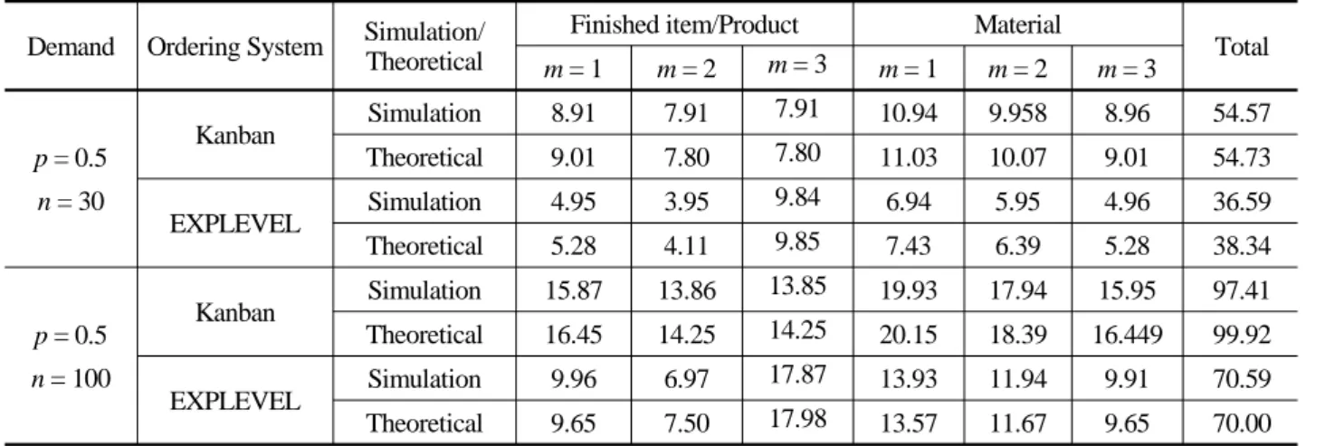
Table 3. Comparison of the EXP + LEVEL system with the Kanban system
Demand Ordering System Simulation/Theoretical
Finished item/Product Material
Total m = 1 m = 2 m = 3 m = 1 m = 2 m = 3
p = 0.5 n = 30
Kanban Simulation 8.91 7.91 7.91 10.94 9.958 8.96 54.57 Theoretical 9.01 7.80 7.80 11.03 10.07 9.01 54.73
EXPLEVEL Simulation 4.95 3.95 9.84 6.94 5.95 4.96 36.59
Theoretical 5.28 4.11 9.85 7.43 6.39 5.28 38.34
p = 0.5 n = 100
Kanban Simulation 15.87 13.86 13.85 19.93 17.94 15.95 97.41 Theoretical 16.45 14.25 14.25 20.15 18.39 16.449 99.92 EXPLEVEL Simulation 9.96 6.97 17.87 13.93 11.94 9.91 70.59 Theoretical 9.65 7.50 17.98 13.57 11.67 9.65 70.00
Table 4. Total inventory for each of ten simulation runs when n = 30
Run No. 1 2 3 4 5 6 7 8 9 10
Kanban 54.44 55.36 53.63 55.52 54.89 54.18 54.94 53.99 53.47 55.28 EXPLEVEL 36.42 37.50 35.48 37.65 36.96 36.16 37.02 35.91 35.34 37.43 Reduction 33.1% 32.3% 33.8% 32.2% 32.7% 33.3% 32.6% 33.5% 33.9% 32.3%
between the two systems due to their sensitivity to the initial stock, we will ignore that difference and compare the performance of the two systems based on the average total inventory. With n = 30 for the binomial distribution for demand in <Table 3>, the average total inventory is reduced from 54.57 in the Kanban system to 36.59 in the EXPLEVEL with
= 0.2. This means that by leveling the pro- duction order quantity under the EXPLEVEL sys- tem, the average total inventory is reduced by 33.0% with a 95% confidence interval of [32.50%, 33.43%] based on the last row in <Table 4>.
With
= 100 for the binomial distribution, the average total inventory is reduced from 97.41 for the Kanban system to 70.59 for the EXPLEVEL system, a 27.5% reduction, in the simulation as shown in <Table 3>.
5.4 Optimal Value of
We will now discuss the optimal value of
which minimizes the expectation of total inventory over all stages of the system. Since it is difficult to realize a predetermined stock-out rate precisely in the simulation as mentioned earlier, our dis- cussion will be based on the theoretical values computed by (23), (24), (27) and (28). This will also allows us to depict the smoothing curves in
the following figures.
<Table 5> gives the expectation of inventory lev- el theoretically computed at the end of period at each stock point for each value of
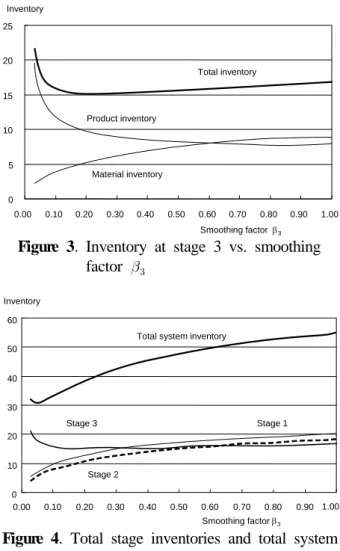
, when the average and variance of the demand are 15 and 7.5, respectively. <Figure 3> and <Figure 4> are depicted based on the values given in the table.
<Figure 3> shows the changes in product inven- tory, material inventory and the total inventory at stage 3 as the smoothing factor
is changed.
<Figure 4> shows the changes in total inventory at each stage as well as the total system inventory as
is changed. Note that the EXPLEVEL system is equivalent to the Kanban system when
= 1.0.
From these tables and figures we can draw the fol- lowing conclusions:
a) Total inventory at the final stage obtained the-
oretically seems to be convex as shown in <Figure
3> and it has a minimum value at around
= 0.2
in this example. The total inventories obtained by
simulation are 16.36 (4.9%), 14.80 (5.5%) and
14.83 (5.2%), when
equals 0.1, 0.2 and 0.3,
respectively. Values in the parentheses are stock-
out rates of the product. The corresponding theoret-
ical values for the total inventories are 16.02,
15.13 and 15.20. When
equals 0.2, the theoret-
ical total inventory at the final stage is 16.81 for
Kanban system as compared to 15.13 for the EXPLEVEL system, which is a reduction of 10.0%.
b) From (23) and (27) we can see that optimal value of
changes according to the production and material replenishment lead-times, but is not influenced by the variability of the demand distri- bution.
c) The average total inventory over the entire system is reduced when
is reduced. The mini- mum value for the average total system inventory is achieved when
= 0.04 as shown in the last column of <Table 5> and in <Figure 4>. From the values given in the last column of <Table 5>, we can see that the total system inventory is reduced from 54.73 at
= 1.0 (Kanban system) to 31.05 at
= 0.04, i.e. 43.3% reduction is obtained. For
n = 100, although any data is not shown, the totalsystem inventory is reduced from 99.92 at
= 1.0 (Kanban system) to the minimum value of 56.59 at
= 0.04 for the EXPLEVEL system, i.e. the same reduction rate as 43.3% is achieved.
Table 5. Average inventory by stage for different
values
Finished
item/Product Material
Total m = 1 m = 2 m = 3 m = 1 m = 2 m = 3 0.03 2.18 1.65 19.59 3.24 2.71 2.18 31.56 0.04 2.51 1.90 17.30 3.71 3.12 2.51 31.05 0.05 2.80 2.12 15.77 4.12 3.46 2.80 31.07 0.06 3.05 2.31 14.66 4.48 3.77 3.05 31.33 0.07 3.28 2.49 13.81 4.81 4.06 3.28 31.74 0.08 3.50 2.66 13.14 5.11 4.31 3.50 32.21 0.09 3.70 2.82 12.59 5.38 4.55 3.70 32.73 0.10 3.88 3.296 12.14 5.63 4.77 3.88 33.26 0.20 5.28 4.11 9.85 7.43 6.39 5.28 38.34 0.30 6.23 4.93 8.96 8.52 7.42 6.23 42.30 0.40 6.93 5.57 8.50 9.25 8.15 6.93 45.33 0.50 7.47 6.10 8.22 9.75 8.67 7.47 47.69 0.60 7.90 6.54 8.05 10.12 9.07 7.90 49.58 0.70 8.24 6.92 7.93 10.41 9.39 8.24 51.12 0.80 8.53 7.24 7.86 10.64 9.64 8.53 52.44 0.90 8.78 7.54 7.82 10.85 9.87 8.78 53.62 1.00 9.01 7.80 7.80 11.03 10.07 9.01 54.73
0 5 10 15 20 25
0.00 0.10 0.20 0.30 0.40 0.50 0.60 0.70 0.80 0.90 1.00 Total inventory
Product inventory
Material inventory Inventory
Smoothing factor β3
Figure 3. Inventory at stage 3 vs. smoothing factor
0 10 20 30 40 50 60
0.00 0.10 0.20 0.30 0.40 0.50 0.60 0.70 0.80 0.90 1.00 Total system inventory
Stage 3 Stage 1
Stage 2
Smoothing factor β3 Inventory
Figure 4. Total stage inventories and total system inventory vs. smoothing factor
5.5 Total Inventory Holding Cost
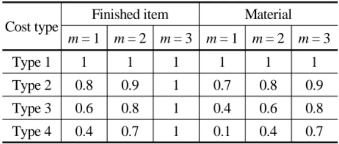
Now consider the total inventory cost reduction by production smoothing. As in most literature, we will use the average inventory at the end of period to evaluate the inventory holding cost. We will thus compute the total inventory cost by multi- plying the average inventory and its unit holding cost together at each stage. We will use four types of unit holding costs as in <Table 6>. For exam- ple, in cost type 4 the unit holding cost of raw material is 0.1 while the unit holding cost of prod- uct at the final stage is 1.0. It is assumed in the table that the same items located at two stock points between two successive stages m and m + 1 have the same unit holding cost.
Using unit costs as shown in <Table 6>, the to- tal inventory holding cost is computed given in
<Table 7>. Since cost type 1 has been used in the
earlier tables, the total inventory cost for cost type
1 is identical to the last column of <Table 5>. The
smallest value of the total inventory cost for each cost type is shown with “*” in <Table 7>. The maximum cost reduction for each cost type for the EXPLEVEL system as compared to the Kanban system (
= 1) is shown in the last row of the table. From <Table 7> we conclude as follows:
a) As the unit material holding cost decreases from type 1 to type 4, overall system inventory cost reduction achieved by the EXPLEVEL system in comparison to the Kanban system goes down from 43.3% to 26.0%.
b) Optimal value of
is 0.04 for cost type 1 while 0.10 for cost type 4. In other words, smaller Table 6. Types of unit inventory holding cost values
used in experiments
Cost type Finished item Material m = 1 m = 2 m = 3 m = 1 m = 2 m = 3
Type 1 1 1 1 1 1 1
Type 2 0.8 0.9 1 0.7 0.8 0.9
Type 3 0.6 0.8 1 0.4 0.6 0.8
Type 4 0.4 0.7 1 0.1 0.4 0.7
Table 7. Total inventory cost for different types of unit holding costs
Cost type 1 Cost type 2 Cost type 3 Cost type 4 0.03 31.56 29.22 26.89 24.56 0.04 31.05* 28.37 25.69 23.01 0.05 31.07 28.09* 25.11 22.13 0.06 31.33 28.09 24.84 21.59 0.07 31.74 28.25 24.76* 21.27 0.08 32.21 28.50 24.79 21.09 0.09 32.73 28.81 24.90 20.99 0.1 33.26 29.16 25.05 20.95*
0.2 38.34 32.84 27.33 21.83
0.3 42.30 35.90 29.49 23.09
0.4 45.33 38.29 31.25 24.21
0.5 47.69 40.18 32.67 25.16
0.6 49.58 41.70 33.83 25.95
0.7 51.12 42.96 34.80 26.63
0.8 52.44 44.04 35.64 27.23
0.9 53.62 45.01 36.39 27.78
1.0 54.73 45.92 37.11 28.31
Reduction 43.27% 38.84% 33.28% 25.98%
the material unit holding cost, larger the optimal value of
.
c) Optimal value of
which minimizes the total inventory holding cost at the final stage is 0.2 for cost type 1 while it is 0.3 for cost type 4 at which 5.54% cost reduction is achieved at the final stage.
5.6 Application to a Supply Chain Manage- ment
The Kanban system is an effective tool to con- trol the production and inventory in a supply chain.
The smoothing of production at the final stage as in the EXPLEVEL system can improve the per- formance of the Kanban system significantly as we have shown in this paper. Consider a supply chain consisting of three different companies, which cor- respond to the three stages in the paper. When a parent company corresponding to the final stage (final assembly station) produces a finished product using production smoothing at
= 0.2, the inven- tory level in the parent company is minimized. At the same time, the other companies composing the supply chain, which would correspond to stages 1 and 2 in the paper, will also reduce their inventory levels and inventory cost owing largely to the pro- duction smoothing at the parent company.
Thus, a win-win relation between companies in a supply chain will be attainable by production smoo- thing at the final assembly company. Although there exists much research concerning quantitative approaches to supply chain management, e.g. Klose
et al. (2002) Graves and Willems (2003) and Dudek(2004), insofar as we know, there may be no way to reduce the total inventory in the supply chain as much as can be achieved by smoothing production at the final stage as shown by the EXPLEVEL system.
6. Conclusion
In this paper, a new ordering policy EXPLEVEL,
in which the production order quantity is leveled
using an exponential smoothing factor, was dis-
cussed for a multi-stage production system. In this
research, we smoothed the production order quan- tity only at the final stage while for the other stages, the production order quantities and material replen- ishment quantities were set according to the Kanban rule.
The contributions of the paper can be summar- ized as follows : (1) Approximations of average in- ventories both for the finished item and the materi- als were derived theoretically. (2) By carrying out simulations, the accuracy of approximations was examined at each stage. Approximations were rela- tively accurate although stock-out rates realized in the simulation are smaller than the pre-set value especially for the materials. (3) The EXPLEVEL system resulted in much lower total inventory cost in a three-stage production and inventory system as compared to the Kanban system. For the produc- tion and inventory systems with more than three stages, smoothing production should be even more effective for inventory reduction. (4) For a wide rage of unit inventory holding costs a smoothing factor smaller than 0.1 leads to the best results in reducing the total inventory cost for the entire pro- duction system. Reducing the smoothing factor im- pacts the total inventory cost reduction at stages 1 and 2 much more than at the final stage. (5) If a parent company using JIT uses production smooth- ing at the final assembly stage and the suppliers manage their production and inventory according to the Kanban rule, then the parent company as well as the suppliers will incur lower inventory holding costs. Thus production smoothing by the parent company, as demonstrated by this paper through the EXPLEVEL system, would result in lower total inventory cost for the entire supply chain, a win- win situation for all the players in the supply chain.
References
Dudek, G. (2004), Collaborative planning in supply chain:
A negotiation-based approach, Springer.
Graves, S. C. and Willems, S. P. (2003), Supply chain Design : Safety stock placement and supply chain config- uration, in de Kok, A. G. and Graves, S. C (Eds.), Hand- book in Operations Research and Management Science Vol.11, Elsevier, 95-132.
Klose, A, Speranza, M. G. and Van Wassenhove, L. N.
Eds. (2002), Quantitative approaches to Distribution lo- gistics and supply chain management, Springer.
Korkmazel, T. and Meral, S. (2001), Bicriteria sequencing methods for the mixed-model assembly line in just-in- time production systems, European J. of Operational Research 131(1), 188-207.
Kotani, S. (1990), Analysis of Kanban System by the Ex- ponential Smoothing Method, Proceedings of 1st APORS within IFORS, 305-318.
Krajewski, L. J., King, B. E., Ritzman, L. P. and Wong, D. S. (1987). Kanban, MRP, and shaping the manufactu- ring environment, Management Science 33(1), 39-57.
Kubiak, W. (1993), Minimizing variation of production rates in just-in-time systems : a survey, European J. of Oper- ational Research 66, 259-271.
Miltenburg, J. (1997), Comparing JIT, MRP and TOC, and embedding TOC into MRP, International Journal of Production Research 35(4), 1147-1169.
Monden, Y. (1998), Toyota Production System : An Inte- grated Approach to Just-In-Time, 3rd Ed., Engineering &
Management Press.
Spearman, M. L., Woodruff, D. L. and Hopp, W. J. (1990), CONWIP : A pull alternative of kanban, International Journal of Production Research 28(5), 879-894.
Tamura, T., Kojima, M., Fujita, S. and Kumagai, C. (2005), An effectiveness of an exponentially smoothed ordering policy, Proceedings of Int. Conference on Operations and Supply Chain Management, Bali-Indonesia, B.1-B.8.
Tamura, T., Dhakar, T. S., Ohno, K. and Kojima. M. (2006), Effectiveness of an Exponentially Smoothed Ordering Policy in a Multi-Stage Production System, Proceedings of the 7th Asia Pacific IE and Management Systems Con- ference 2006, Bangkok-Thailand, 1959-1970.