* 서울과학기술대학교 기계공학과 ([email protected]) 주소: 139-743 서울시 노원구 공릉2동 172
+ 서울과학기술대학교 기계공학과
++ Tamagawa University, Department of Mechanical Engineering +++ 조선대학교 기계설계공학과
++++ The Pennsylvania State University, Department of Engineering Science and Mechanics
Evaluation of Material Properties in Austenite Stainless Steel Sheet with Scanning Acoustic Microscopy
Tae-Sung Park+, Yukio Kasuga++, Ik-Keun Park*, Kyoung-Suk Kim+++, Chiaki Miyasaka++++
(논문접수일 2011. 03. 24, 수정일 2011. 12. 22, 심사완료일 2011. 12. 23)
초음파현미경을 이용한 오스테나이트 스테인레스강의 재료특성 평가
박태성+, Yukio Kasuga++, 박익근*, 김경석+++, Chiaki Miyasaka++++
Abstract
Austenite stainless steel 304 has properties of high resistance to corrosion and temperature changes. Therefore, this material is widely used in various of industries. However, when the material is subjected to heating and cooling cycles the forming accuracy, for example, the right angle associated with a sharp bend such as corner is lost. This phenomenon is caused by the reversion of the deformation-induced martensite into austenite when the temperature in increased. This result in misfit of a structure or an assembly, and an increase in residual stress. Hence, it is important to understand this process.
In this study, to evaluate the mechanical behavior of the deformation-induced martensite and reversed austenite, a scanning acoustic spectroscope including the capability of obtaining both phase and amplitude of the ultrasonic wave (i.e., the complex V(z) curve method) was used. Then, the velocities of the SAW propagating within the specimens made in different conditions were measured. The experimental differences of the SAW velocities obtained in this experiment were ranging from 2,750 m/s to 2,850 m/s, and the theoretical difference was 3.6% under the assumption that the SAW velocity was 2,800 m/s.
The error became smaller as the martensite content was increased. Therefore, the SAW velocity may be a probe to estimate the marternsite content.
Key Words : V(z) curve(V(z) 곡선), Scanning acoustic microscopy(초음파현미경), Surface acoustic wave velocity(표면파속도)
1. Introduction
Austenite stainless steel 304 has the properties of high resistance to corrosion and temperature changes. Therefore
this material is widely used as various industrial applications (e. g., vessels, automobile parts, heat exchangers, electric parts, a like this)(1~2). However, when the material is subjected to heating and cooling cycles the forming accuracy, for
Fig. 1 Schematic diagram of MEDM system example, the right angle associated with a sharp bend such
as a corner is lost(3). This phenomenon is caused by the reversion of the deformation-induced martensite into austenite when the temperature is increased. This results in the warping or misfit of a structure or an assembly, an increase in residual stress, and possible loss of contact members, such as trusses or beams. Therefore, it is important to understand and predict this process. When the martensite reverses into austenite, the timing and affected volume varies with para- meters, such as the stability of the austenite, the elongation and the reversing temperature. Therefore a critical need arises for the mapping of the extent of metallurgical changes on a spot by spot basis. The scanning acoustic microscopy has been successfully developed into an effective microprobe(4). The hypersonic character is especially important because it implies a frequency range from 100 MHz to 2.0 GHz which in turn implies not only high resolution not available with conventional acoustic microscopes and but also microprobe capability. Especially with progress in the interpretation of the so-called V(z) signature(5~7), the SAM has been applied successfully for the measurement of the elastic modulus of materials(8~11), and the mapping of residual stress(12~17) in a typically small region of about 50 micrometer in radius.
However, the application of SAM to measurements on stainless steel was found difficult because of the high absorption of hypersonic waves in the material(18).
In this study, in order to evaluate the appearance of the deformation-induced martensite and reversed austenite, a scanning acoustic microscopy was used. In the experiments, first, axial tension was applied to the stainless steel sheet specimen so as to produce elongation induced martensite, followed by the heat treatment to reverse the martensite into austenite. Second, the martensitic content was measured with Feritscope(19). Finally, using the scanning acoustic microscopy was used to measure and map the SAW velocities. The correlation between the SAW velocities and the degree of deformation was mapped. The measured SAW velocity values were compared and found to be in good agreement with values calculated from the literature.
2. Experimental Apparatus
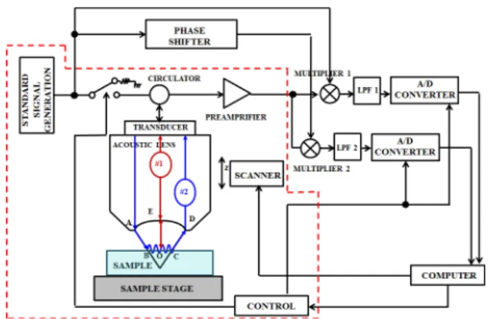
Fig. 1 shows a schematic diagram of scanning acoustic spectroscope (Olympus; model: EPA02; prototype). In this
construction, a standard signal generator for generating a continuous wave of predetermined frequency ranging from 100 MHz~1.0 GHz is connected to an input-side terminal of and analog switch for extracting part of the standard signal and outputting the extracted part as a burst wave one of the output-side terminals of the analog switch is connected to a transducer for subjecting the burst wave to the electro- acoustic conversion and a preamplifier via a circulator. An acoustic lens for converging an ultrasonic wave into a small spot is attached to the transducer. An output terminal the preamplifier is connected to two multipliers. One is directly connected to the standard signal generator so as to receive the standard signal as a reference signal. The other is connected to the standard signal generator via a 90° phase shifting section for generating a reference signal whose phase is shifted by 90° with respect to the standard signal. The output terminals of the multipliers are respectively connected to low-pass filters (LPFs) for removing high frequency components.
The computer is connected to a control section for controlling the distance between the sample and the acoustic lens in the Z axis direction.
3. Theory
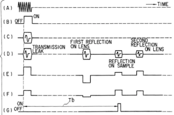
3.1 Measurement of Phase and Amplitude Fig. 2 shows the timing chart to explain the operation. As show in Fig. 2(A), the standard signal generator always generates a continuous wave of constant frequency. When receiving a transmission trigger from the computer, the control section supplies a rectangular signal having a time width corresponding to several tens of periods of the
Fig. 2 The timing chart for illustrating the operation
frequency of the standard signal shown in Fig. 2(B) to the switching terminal of the analog switching terminal of the analog switch in synchronism with the transmission trigger.
The switch effects the switching operating in response to input rectangular signal and the standard signal is output to the circulator only when the switch is set in the ON state.
Thus, a transmission burst signal as shown in Fig. 2(C) is created. The transducer subjects the received transmission burst wave to the electro-acoustic conversion to converts the same into an ultrasonic wave is transmitted via the acoustic lens. The multiplier 1 multiplies the received signal by the received signal by the standard signal to output an in-phase component. multiplier 2 multiplies the received signal by a signal whose phase is shifted by 90° with respect to the standard signal by the phase shifting section to output a quadrature-phase component.
Assume that the standard signal is lagged behind that of the transmission wave because of the elastic property of the sample and time required for propagation in the acoustic lens and the coupler liquid. Assuming that the phase lag is
, the received signal can be expressed by , where B indicates the strength of the received signal.
As a result, the in-phase output from the multiplier 1 and the quadrature-phase from the multiplier 2 can be respectively expressed by the following Eqs. (1) and (2).
coscoscossinsin (1)
sinsincoscossin (2) In this case, since is constant and sin and cos are
also constants, the outputs and contains a D. C.
component and a frequency component of , and therefore, if the component of is removed, sin and cos components (sin and cos) associated with the phase lag of the received signal can be derived.
The components can be removed from the in-phase output from the multiplier 1 and the quadrature-phase output from the multiplier 2 by the LPFs 1 and 2 respectively, and D. C. components corresponding to sin and cos are left behind. The received signal before detection is shown in Fig.
2(D), and the detected outputs of in-phase and quadrature- phase which have passed through the LPFs 1 and 2 are respectively shown in Fig. 2(E) and 2(F).
However, the actual received signal contains reflection waves caused by the transmission leak, first reflection on the lens and second reflection on the lens in addition to the reflection wave caused by the reflection on the sample as shown in Fig. 2(D). Further, since the reflection wave is a burst wave, the phase-detected outputs are generated in the form of a rectangular wave corresponding to the reflection waves as shown in Fig. 2(E) and 2(F). A trigger signal which is delayed by delay time Tb with respect to the transmission wave as shown in Fig. 2(G) is created in the control section and is used as a trigger signal for driving the A/D converter so as to extract only that of the reflection waves which is caused by the reflection on the sample. The detected outputs of in-phase and quadrature-phase are subjected to the A/D conversion by use of the above trigger signal, and after only the phase-detected output caused by the reflection on the sample is converted into digital signal, it is stored into a memory of the computer. The delay time Tb between the transmission signal and the trigger signal for A/D conversion can be freely set to a desired value by means of the computer. The phase and reflection strength are derived based on sin and cos of the stored sample- reflection signal. The Z-scanning section effects the adjusting operation such as focusing operation by changing the distance between the acoustic lens and the sample in response to an instruction from the computer.
Thus, according to the instruction, not only the strength but also the phase can be measured by subjecting the sample-reflection signal to the quadrature detection by use of the standard signal and a signal which is shifted by 90°
with respect to the standard signal.
Fig. 3 Schematic diagram of the SAW propagation
Fig. 4 Example of the V(z) curve 3.2 Measurement of SAW velocity
Fig. 3 shows a schematic diagram of Surface Acoustic Wave propagation between the acoustic lens and the specimens via a coupling medium (e. g., de-ionized water).
When the acoustic lens is moved toward the specimen, the voltage of the transducer changes. The plot of the changes is the so-called V(z) curve. The V(z) curve is formed by the interference at the transducer between normally reflected bulk waves and bulk waves radiated from leaky surface acoustic waves generated from bulk waves impinging onto the sample at the second critical angle.
Fig. 4 shows example of the V(z) curve. The specimen is the silica glass. The temperature of the coupling medium (i.e., de-ionized water) is 23 ℃. The operating frequency of the acoustic lens (Olympus: model; AL4M631) is 400MHz.
The velocity of the SAW is expressed as Eq. (3) from the spacing of the minima ∆ in Fig. 4(20).
∙ ∆ ∙
(3)
where is the velocity of a surface acoustic wave propagating on the specimen, is the velocity of the longitudinal wave of the coupling medium, and is the frequency of the ultrasonic wave emitted from the acoustic lens.
3.3 Accuracy of SAW Velocity Measurement The spherical acoustic lens was used for the measurements of the surface wave velocity. Assuming that ≫
∆
, Eq.
(3) may be expressed as follows:
≅∙ ∙ ∆ (4)
In order to enhance the precision of the SAW velocity measurement by the V(z) curve technique, both sides of Eq.
(4) are differentiated after taking logarithms of both sides.
Then, the following equation is obtained;
∆∆ (5)
Equation (5) shows that the errors in the measurement of the SAW velocity are the sum of the errors in the values of the velocity of the coupling medium, the frequency of the acoustic wave, and the distance of the period. Therefore, in order to minimize the measurement error, it is necessary to maintain a constant temperature for the coupling medium to stabilize the frequency of the acoustic wave, and measure accurately the movement of the acoustic lens along the Z-axis. The frequency of the electrical signal (i.e., tone-burst wave) generated from the transmitter was 600 MHz. The network analyzer (Agilent Technologies; model: 8753D) was used to confirm the stability of the frequency. Measurements were performed in a chamber at constant temperature of 293 K. The specimen was located on the bottom of a glass tank containing the coupling medium (i.e., distilled water). Before measuring the SAW velocity, the specimen was kept in the water tank for several hours to stabilize the temperature at 293 K. In addition, the temperature was monitored by a thermocouple during the experiment. The distance of movement of the acoustic lens along Z-axis was monitored by a laser displacement measuring system (Agilent Technologies; model:
HP5508A) to reduce the error caused by the non-linearity of the movement. Its precision was 10 nm. In the experiments,
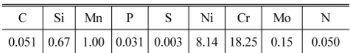
Table 1 Chemical composition of material (mass %)
C Si Mn P S Ni Cr Mo N
0.051 0.67 1.00 0.031 0.003 8.14 18.25 0.15 0.050
Fig. 5 Effect of elongation on martensite content
Fig. 6 Change in martensite content (Tf =273K)
Fig. 7 Martensite content after annealing (λ=10%) nine different localities were randomly selected for determining
the SAW velocity on each specimen and the measurements were repeated three times at each point. The values were obtained from the V(z) curve with the help of a Fast Fourier algorithm.
4. Description of Specimen
The austenitic stainless steel sheets (SUS304) were used.
The chemical compositions are shown in Table 1. The deformation-induced martensite was produced by applying axial tension to strip sheet samples typically having thickness 1.0 mm, width 10 mm and length 120 mm. The ram speed was 4.58 mm/s and the range in elongation was from 5%
to 40%. The ambient temperature Tf was assigned to be 83 K, 203 K, 273 K and 293 K by dipping into liquid nitrogen, dry ice, ice water, and running water, respectively. The temperatures were measured with a precision of ±1.0 K. The elongated specimens were annealed in vacuum. Heating and cooling rates were 5.6 and 1.4 K/min, respectively. The annealing time was 30 min. Annealing temperatures Ta were chosen to be 623, 823, 1023 and 1223 K. Specimens were cut carefully into 3 pieces by high speed disk cutter during wet condition. The specimen surfaces were ground with carborundum paper of successively finer grades down to
#1200. This was followed by polishing successively with 1.0 μm and 0.25μm diamond paste for the final stage. The specimens were then etched for about 10~15 minutes by dipping them into a combined solution of 20 ml ethanol, 80 ml hydrochloric acid and 1.0 g picric acid.
5. Experimental Results
Fig. 5 shows the relationship between the degree of elongation and the martensite content when the temperature was changed. As the elongation is increased, the martensite content is also increased proportionally. The lower the temperature, the larger is the increase in martensite content with the elongation unchanged. This shows that the martensite content is dependent upon both the temperature during
elongation and the degree of elongation itself.
Fig. 6 shows the change in martensite content when the sheet was elongated at Tf=273 K and annealed. The values at Ta=273 K are the values when the sheet is not annealed.
No change in martensite content can be seen up to Ta=823 K. When the annealing temperature was gradually increased, the content of martensite was decreased. Furthermore, the content became almost zero at Ta=1223 K. It means that the
(a) Amplitude
(b) phase
Fig. 8 Example of complex V(z) curve
(a) Amplitude
(b) phase
Fig. 9 Reflectance function versus incident angle
Fig. 10 Effect of elongation on Rayleigh wave velocity deformation-induced martensite is completely reversed back
into the austenite.
Fig. 7 shows the remaining martensite content when the specimen was annealed after the elongation (10%). The martensite content decreased as the annealing temperature was increased. When the temperature was more than 1023 K, almost no martensite remained. This observation suggests that the deformation-induced martensite is almost completely changed into austenite. Martensite content was significantly increased with the temperature at 1223 K. These results match the results shown in Fig. 6.
Fig. 8 shows an example of the complex V(z) curve. Both the intensity and the phase changed periodically with the decrease in the defocusing distance from -50 μm to 0 μm.
Fig. 9 shows the reflectance function versus incident angle.
The minimum value of the amplitude is at around 30° of the incident angle. The phase changes from negative to positive at the Rayleigh critical angle.
Fig. 10 shows the change in SAW velocity due to the elongation. The error in the velocity value obtained in the experimental is at most ±50 m/s and the relative error is 3.6% under the assumption that the velocity is 2800 m/s.
This error became smaller as the martensite content in- creased. The velocity increased as the elongation increased.
At temperatures Tf=83 K and 293 K, a monotonic increase in velocity could not be observed.
When Tf was 293 K, the martensite content was found to be below 10% regardless of the elongation up to 30%. This is seen to lead to the small change in velocity. When Tf is 83 K, consideration and compensation of the thickness is not enough in obtaining the true martensite content from the reading of the Feritscope. Actually more martensite than the result in Fig. 10 is thought to appear. If this were accurately estimated, martensite would be seen to accumulate sufficiently, even with the lower elongation.
6. Discussion
The experimentally obtained SAW velocity was compared to the values calculated from the published elastic pro-
Fig. 11 Measured density, Young’s modulus and Poisson’s ratio
Fig. 12 Comparison of SAW velocity values
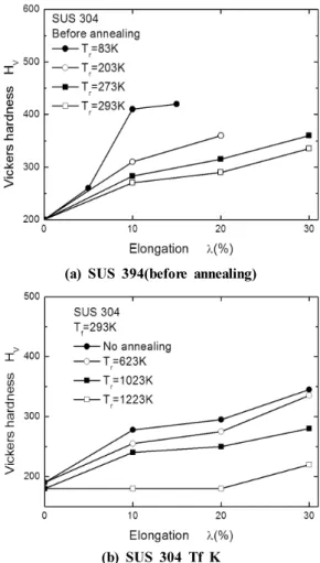
(a) SUS 394(before annealing)
(b) SUS 304 Tf K
Fig. 13 Vickers hardness distribution perties. The longitudinal and shear wave velocities can be
expressed as follows:
(6)
(7)
where, is the velocity of the longitudinal wave, the transverse one, Young's modulus, Poisson's ratio and density.And the relationship among , and is expressed as follows:
(8)Equation (8) can be transformed using Eqs. (6) and (7) when Poisson's ratio is given, and can be obtained. For
example, when is 0.3, . This means that the value for the SAW velocity can be obtained when Young's modulus and density are known in addition to Poisson's ratio. The strip sheets after elongation and annealing were used to obtain Young's modulus and Poisson's ratio. On the surface of the strip sheet, a two-axis rosette strain gauge was adhesive-bonded and the strip was elongated within the elastic range. The density of the material was measured with a densitometer (Model JIS-Z8807). The experimental results are shown in Fig. 11. The change in Young's modulus with annealing temperature is the biggest, followed by the density and Poisson's ratio. When changing values of Tf, the same results were obtained. The change in Poisson's ratio may be considered to be small or negligible throughout the ex- periments. The density was found to increase as the annealing temperature was increased. Austenite has a face-centered- cubic structure, whereas the deformation -induced martensite
′ has a body-centered-cubic structure. As the reversion advanced, the reversed also increased, which implies that
the volume decreased and consequently the density in- creased. In contrast, Young's modulus decreased as the annealing temperature was increased. The results agree well with the ones obtained by Hirayama et al.(21).
Fig. 12 shows good agreement between the calculated SAW velocity and the measured one for EPA02 (prototype).
At first, the change in density due to the deformation-induced transformation was assumed to be related to the change in SAW velocity. The velocity has proved to depend on the change in density and Young's modulus. Vickers hardness was measured as a destructive method in order to support the scanning acoustic microscopy method used for the evaluation of the transformation process of the metastable stainless steel.
Fig. 13 shows that the material hardened as the deformation- induced martensite was increased. Fig. 13 also shows that the hardness increased with the elongation of material. the hardness value grew to over 400, when the ambient temperature was 83 K, which means that the compensation for the thickness in Fig. 3 was incorrect. The results in Fig. 11 agree with the results in Fig. 8: a small increase. Although only the results before annealing are shown, they support the validity of the method for measuring the SAW velocity.
7. Conclusion
Deformation-induced transformation and reversion pro- cesses of stainless steel were evaluated with the Feritscope, hypersonic microscope and acoustic spectrometer. Stainless steel 304 strip sheets of 1 mm thickness were elongated and then annealed. The martensite content was measured after elongation by axial tension and annealing; effects of elongation, ambient temperature and annealing temperature were examined.
Afterwards the surface acoustic wave (SAW) velocity values were obtained by the complex V (z) method at a variety of conditions. The following important conclusions could be ascertained. The lower the ambient temperature, the larger the elongation and the lower the stability of the material, the more martensite appeared. After annealing, the martensite content decreased as the deformation-induced martensite underwent the reverse on process. The calculated SAW velocity agrees well with that measured with scanning acoustic microscopy. This demonstrates usefulness of the scanning acoustic microscopy method, which additionally
was also confirmed by hardness testing. Furthermore, it is possible to estimate the extent of the transformation process for stainless steel with scanning acoustic microscopy, if the SAW velocity changes due to the deformation-induced martensite were separated from the ones due to the reversion process.
Acknowledgment
This work was supported by the National Research Foundation of Korea (NRF) grant funded by the Korea government (MEST) (No. 2011-0017970) (No. 2011-220-D00002).
This work was supported by the Innovations in Nuclear Power Technology (Development of Nuclear Energy Technology) of the Korea Institute of Energy Technology Evaluation and Planning (KETEP) grant funded by the Korea government Ministry of Knowledge Economy (No. 2010-1620100070).
The authors thank to Mr. Tomio Endo (Olympus) for help with acoustic microscopy.
References
(1) Yoo, Y. T., Oh, Y. S., Ro, K. B., and Lim, K. G., 2003,
“Comparison of Welding Characteristics of Austenitic 304 Stainless Steel and SM45C Using a Continuous Wave Nd:YAG Laser,” Transaction of KSMTE, Vol.
12, No. 5, pp. 58~67.
(2) Mo, Y. W., Yoo, Y. T., Shin B. H., and Shin, H. H., 2005, “Welding Characteristics on Hear input Changing of Laser Dissimilar Metals Welding,” Transaction of KSMTE, Vol. 15, No. 2, pp. 51~58.
(3) Kasuga, Y., 1996, “Change in Shape of a Cold Formed and Annealed Stainless Steel Sheet and Joining with use of this Change,” J. of Materials Processing Technology, Vol. 60, No. 1, pp. 233~238.
(4) Atalar, A., Quate, C. F., and Wickramasinge, H. K., 1977, “Phase Imaging in Reflection with the Acoustic Microscope,” Appl. Phys. Lett., Vol. 31, No. 12, pp.
791~793.
(5) Weglein, R. D., 1979, “A Model for Predicting Acoustic Materials Signatures,” Appl. Phys. Lett., Vol 34, No.
3, pp. 179~181.
(6) Parmon, W., and Bertoni, H. L., 1979, “Ray Interpretation of the Material Signature in the Acoustic Microscope,”
Electron. Lett., Vol. 15, No. 21, pp. 684~686.
(7) Atalar, A., 1978, “An Angular Spectrum Approach to Contrast in Reflection Acoustic Microscopy,” J. Appl.
Phys., Vol. 49, Issue 10, pp. 5130~5139.
(8) Kushibiki, J., Ueda, T., and Chubachi, N., 1987,
“Determination of Elastic Constants by LFB Acoustic Microscope,” IEEE Ultrasonics Symp. Proc., pp. 817~
821.
(9) Nishida, M., and Endo, T., 1993, “Measurement of Elastic Moduli in Local Area by Scanning Acoustic Microscope,” Proc. Experimental and Theoretical Mechanics, pp. 290~297.
(10) Okade, M., Mizuno, K., and Kawashima, K., 1995,
“Measurement of Acoustoelasti Coefficients of Surface Wave with Scanning Acoustic Microscopy,” Rev. Prog.
Quant. Nondestr. Eval., Vol. 14, pp. 1883~1889.
(11) Okade, M., Hasebe, T., Kawai, T., and Kawashima, K.,
1996, “New Digital Techniques for Precise Measurement of Surface Wave Velocity with Acoustic Microscope,”
Mater. Sci. Forum, Vol. 210-214, pp. 839~846.
(12) Obata, M., Shimada, H., and Mihara, T., 1990, “Stress Dependence of Leaky Surface Wave on PMMA by Line-Focus-Beam Acoustic Microscope,” Exp. Mech., Vol. 30, No. 1, pp. 34~39.
(13) Miyasaka, C., and Tittmann, B. R., 2005, “Acoustic Microscopy Applied to Ceramic Pressure Vessels and Associated Component,” Transactions of the ASME, Vol. 127, pp. 214~219
(14) Miyasakam, C., Tittmannm, B. R., and Tanakam, S., 2002, “Characterization of Stress at a Ceramic/Metal Joined Interface by the V(z) Technique of Scanning Acoustic Microscopy,” Pressure Vessel Technol, Vol.
124, No. 3, 336~342.