논문 2013-50-11-21
스케일 텔레 로보틱스 시스템에 적용된 Routh-Hurwitz와 절대 안정도 기준의 비교
( Comparison of Routh-Hurwitz and Absolute Stability Criteria in Application to Scaled Telerobotics Systems )
이고르 가포노프*, 조 현 찬**, 전 홍 태****
( Igor Gaponov, Hyun Chan Cho
ⓒ, and Hong-Tae Jeon )
요 약
본 논문에서는 스케일 텔레 로보틱스 시스템에 Routh-Hurwitz와 Llewellyn의 절대 안정도 기준의 적용에 관한 비교 연구 결과를 보인다. 텔레 로보틱스 시스템의 동적 방정식이 주어지고, 시스템의 전달함수는 더 나은 안정도 해석을 얻게 된다. 제 어기 이득의 안정적인 마진은 두 가지의 안정도 해석 방법을 통하여 얻을 수 있으며, 본 논문에서 그 결과의 차이를 밝히고 설명했다. 본 논문은 안정도 분석결과를 수치 예제를 통해 증명하는 것으로 결론을 도출한다.
Abstract
This paper presents a comparative study on application of Routh-Hurwitz and Llewellyn absolute stability criteria to a scaled telerobotic system. The dynamic equations of the telerobotic system are given, and the transfer function of the system is obtained for further stability analysis. The stable margins of controller gains are obtained using both stability analysis methods, and the differences in the results are described and explained. The paper is concluded by a numerical example verifying performed stability analysis.
Keywords : telerobotic system, stability, Routh-Hurwitz criterion, Llewellyn absolute stability criterion.
Ⅰ. Introduction
Manipulation of micro- and nanoscale objects is required in many applications nowadays, like intracytoplasmic sperm and DNA injection in living
* 정회원, 한국기술교육대학교 기계공학부
(School of Mechanical Engineering, KoreaTech)
** 정회원, 한국기술교육대학교 전기전자통신공학부 (School of Electrical, Electronics and
Communication Engineering, KoreaTech)
*** 정회원, 중앙대학교 전자전기공학부
(Dept. of Electrical and Electronics Engineering, Chung-Ang University)
ⓒCorresponding Author(E-mail: [email protected]) 접수일자:2013년7월25일, 수정완료일:2013년10월26일
cells, molecular docking, minimally invasive and micro-surgery, and many others. The main reason of the emerging role of micro-telerobotic systems is that they provide the human operator with the feeling of interaction (haptic force) with the micro-environment, while granting the operator an opportunity to be at a remote site while performing required manipulations.
Stability is the fundamental requirement of every control system. In addition, a telerobotic system must provide the operator with an accurate feeling of the environment (be transparent), the condition that usually interferes with stability. To this day, many
bilateral control architectures have been developed and applied to telerobotic systems[1-3]. However, there is still need in guidelines for engineers who perform stability analysis of the scaled telerobotic systems due to the complexity of their structure and uncertainties in human hand and environment parameters.
This paper presents a comparative study of application of Routh-Hurwitz and Llewellyn absolute stability analysis. In Section Ⅱ, the architecture of the proposed control system is described, and the assumptions for further stability analysis are given.
In Section Ⅲ, a comparative investigation of system stability using Routh-Hurwitz and Llewellyn absolute stability criteria is given and verified by a numerical simulation. The paper is concluded by Section Ⅳ.
Ⅱ. Control System Architecture
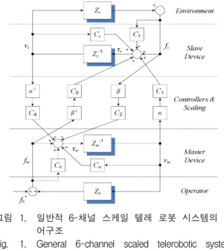
A general 6-channel architecture of a telerobotic control system is presented in Fig. 1. Proposed by Hannaford[4], this architecture was originally 4-channelled (signals between the master and the slave manipulators flow through four controllers (C1,
그림 1. 일반적 6-채널 스케일 텔레 로봇 시스템의 제 어구조
Fig. 1. General 6-channel scaled telerobotic system control architecture.
C
2, C3, C4) and was later extended by Hastrudi-Zaad and Salcudean[5] by adding master and slave local force feedback loops (controllers C5 and C6). It should be also noted that the signals exchanged between master and slave sides are scaled by respective scaling coefficients( and or -1 and -1), whichVariable Description
Master device position
Slave device position
Master device velocity
Slave device velocity
Master device force
Slave device force
Exogenous force of operator 표 1. 안정도 분석에 사용된 변수 리스트 Table 1. List of variables used in stability analysis.
Variable Description
Master device impedance
Slave device impedance
Impedance of environment
Impedance of human operator
Master device controller
Slave device controller
Master position feedforward control
Slave force feedforward control
Master force feedforward control
Slave position feedforward control
Slave local force feedforward
Master local force feedforward
Position scaling coefficient
Force scaling coefficient
표 2. General 6-channel 텔레 로보틱스 구조의 전달 함수
Table 2 Transfer functions of a general 6-channelled Telerobotic architecture.
Transfer Function Form
표 3. 전달함수 내용
Table 3. Descriptions of some transfer functions.
was beyond the scope of the above mentioned works.
In Table 3, parameters m, b, k denote mass, viscosity, and stiffness coefficients of the respective transfer functions, kmv and kmp denote the velocity and position gains of master PD-controller, and ksv
and ksp stand for the velocity and position gains of slave device PD-controller.
In general, the impedance of the operator Zh varies from person to person, and the environment, especially micro-environment, is hard to model exactly in most cases. However, since both operator and environment are passive systems, it is enough to analyze the stability of the two-port network model of the teleoperator only, which includes master device, slave device, and the communication block in Fig. 1.
The hybrid matrix is defined as[4~5]
It can be shown that the elements of the hybrid matrix hij , where i, j = 1, 2, can be found to be[5]
(1)
(2)
(3)
(4)
where Zc+m = Cm + Zm, Zc+s = Cs + Zs..
Adopting force-position (force reflecting) architecture yields C3 = C4 = C5 = C6 = 0. Choosing the remaining controllers to be C1 = C1v + C1p/s and
C
2 = 1, the transfer functions Fh/Fe and F*h/Fe can be obtained as follows:
∙
≡
(5)
The characteristic equation of the transfer function (5) can be expressed in the following form:
∙
(6)
The following assumptions are made in order to simplify the further analysis:kmv, ksv
>> b
m, bh, be, bskmv, ksv
>> m
m, mh, me, mskmp >> bm, bh, be
ksp >> ke
me << mh, mm, ms
Choosing the controllers C1 and C2 to be C1p = ke
+ ksp, C2 = , the coefficients of the polynomial described by (6) can be defined as follows:
∙
(7)
∙ ∙
(8)
∙
(9)
∙ ∙
(10)
∙
(11)
Ⅲ. Stability Analysis
Stability is a critical issue in telerobotics, especially in the presence of time delays. The following techniques are most commonly used to estimate the stability of telerobotic systems:
∙ Routh-Hurwitz criterion
∙ Lyapunov functions-based approach
∙ Nyquist criterion
∙ Llewellyn’s(absolute) stability criterion
∙ Passivity analysis
All of the above mentioned methods are well-known in control theory and have their flaws and benefits. For instance, the Routh-Hurwitz criterion is the simplest and the least computational-demanding technique, however, it does not reflect the nonlinearities existing in the system.
Lyapunov stability approach guarantees the asymptotical stability of the system; however, its applications are restricted due to the difficulties in finding satisfactory Lyapunov function candidates for every particular system. Passivity theory is relatively simple in implementation, but provides conservative.
conditions[6]. Absolute stability criterion (Llewellyn’s criterion) is a less conservative condition compared to passivity, and has gained more popularity among control engineers in recent years.
In this research, two stability criteria, namely the Routh-Hurwitz criterion and Llewellyn’s stability criterion, are applied to analyze the stability of a general scaled telerobotic system. The qualitative comparison between those two criteria is performed, and their restrictions are discussed. The Routh-Hurwitz criterion was chosen due to its simplicity, and the absolute stability criterion was selected as one of the most advanced stability analysis methods that can provide stable margins for controller gains while taking into the account the frequency of the input signal.
1. Routh-Hurwitz Criterion
For a fourth-order polynomial, the Routh-Hurwitz criterion is formulated as follows:
∙ 0;
∙
∙
In order for the first condition to hold, it is necessary that all the parameters used in the mathematical model presented in Section II, namely controllers’ gains and physical properties of the human operator, master and slave devices, and environment, are positive. It is assumed that only the positive values of the above mentioned parameters are used in the further analysis.
The second condition of the Routh-Hurtwitz criterion (a3
a
2 > a4a
1) provides the following stable margins for the regulator gains:
∙ ∙
∙ ∙
∙
(12)
∙
∙ ∙
∙ ∙
(13)
∙
∙
∙
∙
(14)
∙
∙
∙ ∙
∙
(15)
Now it is possible to find the stable margins of the controller gains
k
mv,k
mp,k
sv,k
sp. Using the approximate values of the coefficients of the characteristic equation, the expression (12) can be written as follows: ∙
(16)
Since the values of all the regulator gains andphysical parameters in expression (16) are non-negative, it is possible to conclude that this inequality will hold for all of the non-negative values of kmp. Therefore, we can state that the choice of the value of kmp
gain does not affect the stability of the
system according to the Routh-Hurwitz criterion.Similarly, it can be shown that selecting a non-negative value of ksp
will not result in the
deterioration of system stability, as it follows from (13).Now let us find the stable margins for the ksv
gain. Putting the inequality (14) in the form x2+ bx -
c > 0 and solving it, we obtain the following
boundaries of the ksv gain:
or
where b = ms
[k
mv/(mm + mh) - kmp/kmv], c = msk
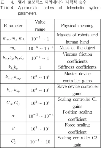
sp. Since we are looking only for the positive value ofParameter Value
range Physical meaning
∼ Masses of robots and human hand
∼ Mass of the object
∼ Viscous friction coefficients
Stiffness coefficients
∼ Master device controller gains
∼ Slave device controller gains
∼ Scaling controller C1 gains
∼ Position scaling coefficient
∼ Force scaling coefficient
∼ Scaling controller C2 gain
표 4. 텔레 로보틱스 파라메터의 대략적 승수
Table 4. Approximate orders of telerobotic system parameters.
the ksv
gain, we are interested only in the second
inequality among those two, or
(17)
From Table 4, we find that the parameters b and c have the order of 103-104; therefore, it can be conjured that b2>>4c. Hence, the minimum stable margin of the ksv
gain, according to inequality (17),
would be a positive value close to zero. Accordingly, we can find that the same conditions apply to the stable range of the kmvgain. Therefore, it can be
stated that choosing the controllers gains kmvand k
svto be positive values of the third or fourth order will not lead to the instability of the control system.
2. Llewellyn’s Criterion
Llewellyn’s criterion for absolute stability is expressed in terms of immitance matrix parameters as follows:
1. z11 and z22 have no poles in the right half plane.
2. Any poles of z11 and z22 on the imaginary axis are simple with real and positive residues. These two conditions can be written in mathematical form as follows:
≥
(18)
≥
(19)
3. The third condition can be written in several ways:
z Llewellyn (1952)
∙
(20, a)
z Hashtrudi-Zaad and Salcudean (2001)
≥
(20, b)
z Adams and Hannaford (1999); Son et al. (2009)
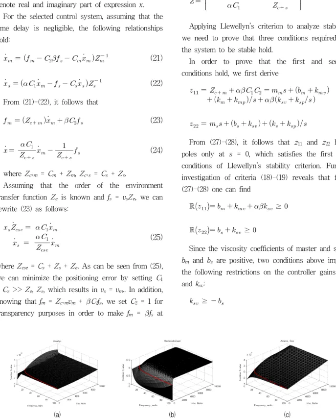
(a) (b) (c) 그림 2. 입력신호 주파수와 이득 ksv의 변화 값의 함수로써 기준 (20, a)-(20, c) 값의 변화
Fig. 2. The values of criteria (20, a)-(20, c) as a function of input signal frequency and various values of the ksv gain.
≥
(20, c)
In the expressions above, the terms and denote real and imaginary part of expression x.For the selected control system, assuming that the time delay is negligible, the following relationships hold:
(21)
(22)
From (21)-(22), it follows that
(23)
(24)
where Zc+m = Cm + Zm, Zc+s = Cs + Zs.
Assuming that the order of the environment transfer function Ze is known and fs = vs
Z
e, we can rewrite (23) as follows:
(25)
where Zcse = Cs + Zs + Ze. As can be seen from (25), we can minimize the positioning error by setting C1
= Cs >> Ze, Zs, which results in vs = vm.. In addition, knowing that fm = Zc+m
v
m + C2f
s, we set C2 = 1 for transparency purposes in order to make fm = fs atthe settled state.
The impedance matrix can be written as follows:
(26)
Applying Llewellyn’s criterion to analyze stability, we need to prove that three conditions required for the system to be stable hold.
In order to prove that the first and second conditions hold, we first derive
(27)
(28)
From (27)-(28), it follows that z11 and z22 have poles only at s = 0, which satisfies the first two conditions of Llewellyn’s stability criterion. Further investigation of criteria (18)-(19) reveals that from (27)-(28) one can find ≥
(29)
≥
(30)
Since the viscosity coefficients of master and slave
b
m and bs are positive, two conditions above impose the following restrictions on the controller gains kmvand ksv:
≥
(31)
≥
(32)
For the sake of convenience of notation, let us introduce the following variables:
(33)
(34)
(35)
(36)
Hence, expressions (29)-(30) will take the following form:
≥
(37)
≥
(38)
The third criterion of Llewellyn’s stability can be investigated by dividing one of the three conditions (20, a-c) into two parts. For instance, for condition (20, c) this may look as follows[7, 8]:
≥
(39)
≥
(40)
Since
(41)
substituting equations (26), (33)-(36), and (41) into (39) and taking values from the Table 3 yields
≥
(42)
Having bs+c ≥ 0 from (38) and assuming bm+c, ksp
≥ 0, we can then prove that the inequality (42) is satisfied for all frequencies of the input signal .
Since both of the viscosity gains of master and slave devices (bm and bs), along with slave mass ms
and
stiffness coefficient ks, are always non-negative
values, we can prove that for the control system to be stable for all real values of , it is required that≥
(43)
≤
(44)
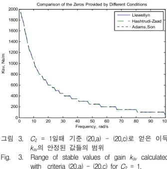
Hence, in order to satisfy the absolute stability criteria, the controller gains should not violate conditions (37)-(38) and (43-44). Similar reasoning can be applied to any of the criteria (20, a) - (20, c), and they will produce the same stable margins of controller gains. Figure 2 presents the values of conditions (20, a) - (20, c) as a function of input signal frequency and controller gain ksv, and Figure 3 shows the values of the gain ksv at which the criteria intersect horizontal axis for input signal frequencies ranging between 0 and 100 rad/s. It can be noted from Figure 3 that the results obtained using different criteria remain equivalent.
We may conclude application of Llewelyn’s absolute stability criteria imposes less conservative stability conditions on controllers gains in comparison
0 10 20 30 40 50 60 70 80 90 100
0 200 400 600 800 1000 1200 1400 1600 1800 2000
Frequency, rad/s
Ksv, Ns/m
Comparison of the Zeros Provided by Different Conditions Llewellyn Hashtrudi-Zaad Adams,Son
그림 3. C2 = 1일때 기준 (20,a) - (20,c)로 얻은 이득 ksv의 안정된 값들의 범위
Fig. 3. Range of stable values of gain ksv calculated with criteria (20,a) - (20,c) for C2 = 1.
to those obtained using the Routh-Hurwitz criterion.
These margins are also frequency-dependent in case of absolute stability criteria.
3. Numerical Example
A numerical simulation has been conducted in order to verify the stability margins obtained above.
The exogenous input force was the unit step with the magnitude of 1 N. The following system parameters have been chosen:
∙ human operator: mh = 1 kg, bh = 0.1 Ns/m, kh= 0 N/m;
∙ master device: mm = 0.7 kg, bm = 0.1 Ns/m;
∙ slave device: ms=1 kg, bs=1 Ns/m;
∙ environment: me=10-6 kg, be=0.1 Ns/m,
k
e=10N/m;∙ master controller: kmv=2000 Ns/m, kmp=10000 N/m;
∙ slave controller: ksv=5000 Ns/m, ksp=15000 N/m;
∙ scaling coefficients: = 10-3, = 2000;
∙ position and force feedforward regulations:
C
1v=5000 Ns/m, C1p=45000 N/m, C2=1.The transient responses of the studied control
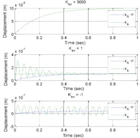
그림 4. 서로 다른 이득 ksv에서의 텔레 로보틱스 시스 템의 계단응답
Fig. 4. Step responses of the telerobotic system under different values of ksv gains.
system for the different values of ksv
gain are shown
in Fig. 4. One can ascertain that as soon as the marginal condition ksv=-bs is met, the system shows oscillatory convergence, which means that it reaches the boundary of stability region (the bottom plot in Fig. 4), and once the condition (29) does not hold, the system diverges. Similar plots confirming the stability analysis conducted above can be plotted for all of the controller gains. It can be noted that the system remains stable even for some negative values of ksv, which is confirmed by the absolute stability criteria but contradicts the Routh-Hurwitz criterion.Therefore, it can be concluded that the Llewelyn’s stability criterion provides less conservative stability margins.
4. Conclusion
In this paper, the outlines on application of Routh- Hurwitz and Llewellyn stability criteria to a scaled Telerobotic system stability analysis are discussed.
The dynamics of the scaled teleoperated system is studied, and the closed-loop transfer function of the system is derived. Next, the Routh-Hurwitz and Llewellyn stability criteria are applied in order to find stable margins of the controller gains of master and slave devices. It is shown that although Routh-Hurwitz criterion is more simple in its application to an actual control system, it gives more conservative conditions on controller gains. In addition, it is possible to obtain less conservative stable gain margins using the Llewellyn absolute stability criteria if the frequency of the input signal is known (lies in a given range). The conducted analysis is confirmed by a numerical simulation.
REFERENCES
[1] B. Hannaford, “A design framework for teleoperators with kinesthetic feedback,” IEEE Tran. on Robotics and Automation, Vol. 5, no. 4, pp. 426–434, 1989.
[2] Y. Yokokohji and T. Yoshikawa, Bilateral
저 자 소 개 이고르 가포노프(정회원)
2006년 러시아 쿠르스크 대학교 메카트로닉스 및 자동화 공학과 공학사
2008년 한국기술교육대학교 기계 공학과 공학석사
2011년 한국기술교육대학교 기계 공학과 공학박사
2011년~현재 한국기술교육대학교 기계공학부 조교수
<주관심분야 : 로보틱스, 제어이론, 텔레로봇시스 템>
조 현 찬(정회원)
1983년 광운대학교 전자공학과 공학사
1985년 중앙대학교 전자공학과 공학석사
1991년 중앙대학교 전자공학과 공학박사
1991년~현재 한국기술교육대학교 전기전자통신 공학부 교수
<주관심분야 : 지능알고리즘 및 시스템제어, 바이 오-전자공학, 로보틱스>
전 홍 태(정회원)
1976년 서울대학교 전자공학과 1986년 뉴욕 주립대학 전기전자공 학과(공학박사)
1986년 9월∼현재 중앙대학교 전자전기공학부 교수
<주관심분야 : 지능시스템, 로보틱스, 시스템 제 어>
control of master-slave manipulators for ideal kinematic coupling Formulation and experiment.
IEEE Trans. on Robotics and Automation, pp.
605– 620, 1994.
[3] S. E. Salcudean, “Control for teleoperation and haptic interfaces”, in Control Problems in Robotics and Automation, LNCIS-230, ed. B.
Siciliano and K. P. Valavanis, pp. 51–66. New York: Springer-Verlag, 1998.
[4] B. Hannaford, “A design framework for teleoperators with kinesthetic feedback,” IEEE Tran. on Robotics and Automation, vol. 5, no. 4, pp. 426–434, 1989.
[5] K. Hastrudi-Zaad, S.E. Salcudean, “On the use of local force feedback for transparent teleoperation”, IEEE Proc. Int. Conf. Robotics and Automation, vol. 3, pp. 1863-1869, 1999.
[6] Jazayeri, A.; Tavakoli, M., “A Passivity Criterion for Sampled-Data Bilateral Teleoperation Systems”, Haptics, IEEE Transactions on, vol. 6, no. 3, pp. 363-369, July-Sept. 2013
[7] H. I. Son, T. Bhattacharjee, H. Hashimoto,
“Enhancement in operator’s perception of soft tissues and its experimental validation for scaled teleoperation systems”, IEEE/ASME Trans. on Mechatronics, vol. 16, issue 6, pp. 1096-1109, 2011.
[8] H. I. Son, T. Bhattacharjee, D.Y. Lee, “Control design based on analytical stability criteria for optimized kinesthetic perception in scaled teleoperation”, ICROS-SICE Int. Joint Conf., pp.
3365- 3370, 2009.