Level Set based Topological Shape Optimization of Phononic Crystals

음향결정 구조의 레벨셋 기반 위상 및 형상 최적설계

김 민 근¹․하시모토 히로시²․아베 카주히사²․조 선 호^3†

1삼성중공업 풍력발전사업부, ²니가타대학교 토목공학과, ³서울대학교 조선해양공학과

Level Set based Topological Shape Optimization of Phononic Crystals

Min-Geun Kim¹, Hiroshi Hashimoto², Kazuhisa Abe² and Seonho Cho^3†

1WTG development team1, Samsung Heavy Industries, Geouje, 656-813, Republic of Korea

2Department of Civil Engineering, Niigata University, Niigata, 950-2181, Japan

3Department of Naval Architecture and Ocean Engineering, Seoul National University, Seoul, 151-744, Republic of Korea

Abstract

A topology optimization method for phononic crystals is developed for the design of sound barriers, using the level set approach.

Given a frequency and an incident wave to the phononic crystals, an optimal shape of periodic inclusions is found by minimizing the norm of transmittance. In a sound field including scattering bodies, an acoustic wave can be refracted on the obstacle boundaries, which enables to control acoustic performance by taking the shape of inclusions as the design variables. In this research, we consider a layered structure which is composed of inclusions arranged periodically in horizontal direction while finite inclusions are distributed in vertical direction. Due to the periodicity of inclusions, a unit cell can be considered to analyze the wave propagation together with proper boundary conditions which are imposed on the left and right edges of the unit cell using the Bloch theorem. The boundary conditions for the lower and the upper boundaries of unit cell are described by impedance matrices, which represent the transmission of waves between the layered structure and the semi-infinite external media. A level set method is employed to describe the topology and the shape of inclusions. In the level set method, the initial domain is kept fixed and its boundary is represented by an implicit moving boundary embedded in the level set function, which facilitates to handle complicated topological shape changes.

Through several numerical examples, the applicability of the proposed method is demonstrated.

Keywords : topological shape optimization, level set method, noise barrier performance, Bloch theorem, acoustic wave transmission, adjoint variable method

†Corresponding author:

Tel: +82-2-880-7322; E-mail: [email protected] Received November 19 2012; Revised November 29 2012;

Accepted December 1 2012

Ⓒ 2012 by Computational Structural Engineering Institute of Korea

This is an Open-Access article distributed under the terms of the Creative Commons Attribution Non-Commercial License(http://creativecommons.

org/licenses/by-nc/3.0) which permits unrestricted non-commercial use, distribution, and reproduction in any medium, provided the original work is properly cited.

1. Introduction

Periodic materials designed for acoustic or elastic wave propagation are called phononic crystals. The significance of these materials results from the band structure with band gaps. Utilization of this property makes it possible to control the wave transmission in the material. Since the capability of such a structure strongly depends on the shape and arrangement of inclusions characterizing the periodicity, it is worth- while to explore an effective layout. Many resear-

chers have attempted to develop acoustic barriers by utilizing the band structure(Qjan et al., 2008; Vasseur et al., 1994). The shape optimization method for the periodically distributed inclusion can be a useful tool for this task(Håkansson et al., 2004). Sigmund and Jensen(2003) tried to find optimal shape of inclus- ions for maximization of the band gap using topology optimization methods.Recently, He et al.(2007) per- formed the level set method incorporating topological derivatives into shape derivatives to obtain layout as well as shape of photonic crystals.

Fig. 1 Acoustic barrier in infinite acoustic field Although periodicity plays an important role in

the insulation of waves, a barrier given by an array of scatters has a finite thickness. Therefore, it is valuable to know how to evaluate the transmitting waves through a barrier with finite thickness in the context of the shape design. Yamada et al.(2010) developed a level set-based topology optimization method for layers of photonic crystals imbedded in an infinite medium. In order to describe the radia- tion condition in semi-infinite domains locating on both sides of the barrier, they replaced the half- planes to finite energy absorbing regions. This appro- ximation needs excessive discretization of these regions to add to the unit layer. Since the optimization analysis involves a number of wave transmission analyses, the extension of the domain size results in the increase of computational cost. Abe et al.

(2010) proposed a transmitting boundary for semi- infinite wave fields synchronized with the perio- dicity of a combined layer, which is applicable not only to homogeneous media but also to periodic structures. This is given by an impedance matrix composed of propagating wave modes. The transmi- tting boundaries are to be coupled with the lower and upper sides of the periodic layer.

In this research, a topological shape optimization method of phononic crystals for sound barrier is developed using level set methods. The purpose of design optimization is to get an optimal shape of periodic inclusions by minimizing the norm of the transmittance at given frequencies and an incident angle of waves attacking the phononic crystals. By deriving impedance matrix to consider transmittance of acoustic energy, we can define energy transmi- ttance instead of band-gap concept as an objective function, and an optimal solution is guaranteed since energy measure is dealt. In this research, a layered structure is considered which is composed by inclusions arranged periodically in the horizontal direction while finite inclusions are distributed in the vertical direction. The distributions of inclusions are already determined and the shape of inclusion is considered as design to control acoustic waves.

The periodic boundary conditions are imposed on the left and right edges of the unit cell in a layer by using the Bloch theorem. The upper and lower ends which are for the transmission of waves between the layered structure and the semi-infinite external media are described by impedance matrices(Abe et al., 2010). Once the impedance matrices have been obtained, one can analyze the wave propagation without any additional degrees of freedom. More- over, since the impedance matrix is independent of the structure of the insulating wall, the recons- truction of the matrices is not required during the optimization process.

To describe complex shape of inclusions, the level set method is employed. In the level set method, the initial domain is kept fixed and its boundary is represented by an implicit moving boundary(IMB) embedded in the level set function, which facilitates to handle complicated topological shape changes.

Furthermore, a material interpolation for scatter and outside of scatters using level set function makes it easy to deal boundary conditions between two different medium without difficulties in phononic crystal structures.

2. Wave transmission analysis

2.1 Acoustic analysis for incident wave

Let us consider a periodic layer consisting of acoustic scatters(inclusions) as shown in Fig.1. The scattering layer rests horizontally on an infinite acoustic field. The periodic length of the arrange-

ment is . The barrier is subjected to anincident wave ^ which propagates to upwards in the lower half-infinite region .

The governing equation of the acoustic wave is given by the following Helmholz equation:

2u( ) 2 u( ) 0

β∇ x +ω ρ x = for x∈Ω (1)

where ^ is the sound pressure, ^ is the acoustic medium, ^ and ^ are adiabatic bulk modulus, material densities, respectively. The adiabatic bulk modulus is defined as ^{  } for ^ the speed of sound and the circular frequency ^. The boundary value on the obstacle is given by:



  on ^ (2)

where ^ stands for the outward normal and ^ is the boundary of the scatteres. For a unit cell of the layer, , the finite element equation is

{ } { }

K uˆ f

⎡ ⎤ =

⎣ ⎦ (3)

where ^ is the nodal vector of the sound pre- ssure, ^ is the flux vector, ^   ^, ^ and ^ are stiffness and mass matrices degene- rated based on the Bloch’ theorem:

L L ik

R e u

u = ¹¹ , f_R =−e^ik1L1 f_L (4)

where ^{ } and ^{ } are sub-vectors consisting of nodes on the left and right sides of the unit cell, respectively. ^ is the horizontal component of a wave vector. In terms of sub-matrices of ^, Equation (3) can be rewritten as

⎪⎪

⎭

⎪⎪

⎬

⎫

⎪⎪

⎩

⎪⎪

⎨

⎧

=

⎪⎪

⎭

⎪⎪

⎬

⎫

⎪⎪

⎩

⎪⎪

⎨

⎧

⎥⎥

⎥⎥

⎥

⎦

⎤

⎢⎢

⎢⎢

⎢

⎣

⎡

0 0 ˆ

ˆ ˆ ˆ

ˆ ˆ ˆ ˆ

ˆ ˆ ˆ ˆ

ˆ ˆ ˆ ˆ

T B

L M T B

LL LM LT LB

ML MM MT MB

TL TM TT TB

BL BM BT BB

f f

u u u u

K K K K

K K K K

K K K K

K K K K

(5)

where ^{ } and ^{ } stand for sub-vectors corres- ponding to the bottom and the top of the unit cell.

 _ indicates the rest component vector. In this problem, we assume that there is no sound source in the domain. In Equation (5), ^ and ^ are unknown sub-vectors. In order to evaluate these unknowns, the compatibility and equilibrium condi- tions at the interfaces between  and , and 

and  can be considered :

{ } { }F2 + f_B =0, { } { }u2 = uB (6)

{ } { }F1 + f_T =0, { } { }u1 = uT (7) where ^{ } and ^{ } are sub-vectors on the interfaces of  and . Consequently, ^_ and ^_ can be replaced by ^ and ^, respectively.The solution in the lower half-plane  represented by a unit cell  is composed of the incident and reflected waves as shown in Fig. 1. The acoustic wave and flux ^ and ^ of  can be decomposed into two terms (Fig. 2(a)) as

{ }^{u1 =}

{ } { }

{ } { }

where the first terms on the right hand side are vectors relevant to the incident wave, while the second terms correspond to the reflected wave. The internal flux for the incident wave ^ can be evaluated by the relation between the nodal acoustic pressure ^ and the nodal flux  at the interface. Since the incident wave is propagating to upwards, this relation can be described for an upper semi-infinite field  complementing to the lower semi-infinite field  (Fig. 2(a)) by

[ ]

_^^_^, the flux of the incident wave is expressed as

{ }

{ }

Fig. 2 Acoustic barrier in infinite acoustic field

where ^ stands for the nodal internal flux acting on the bottom boundary of the upper semi- infinite , excited by the incident wave. Since the reflected wave from the boundary of  travels to downwards (Fig. 2(b) and (c)), it can be described by

{ } [ ]

{ }

R

D K u

F = ₁ (11)

where ^ is an impedance matrix for the top boundary of lower semi-infinite .

In a similar manner, the transmitted wave which propagates in the upper semi-infinite  can be represented by

{ }

[ ]{ }

{ }^{F1 =}[ ]^K1D { }^{u1 −}[^K1U+K1D]

{ }

Using Equations (6), (7), (12) and (13), we can express Equation (5) in terms of the impedance matrices and incident acoustic wave such as

[ ]

{ }

1 1 1

2

ˆ ˆ ˆ ˆ

ˆ ˆ ˆ ˆ 0

ˆ ˆ ˆ ˆ 0

ˆ ˆ ˆ ˆ 0

BB D BT BM BL B U D I

TB TT U TM TL T

MB MT MM ML M

LB LT LM LL L

K K K K K u K K u

K K K K K u

K K K K u

K K K K u

⎡ + ⎤⎧ ⎫ ⎧ + ⎫

⎢ + ⎥⎪ ⎪ ⎪ ⎪

⎢ ⎥ ⎪ ⎪ ⎪⎨ ⎬ ⎨= ⎪⎬

⎢ ⎥

⎪ ⎪ ⎪ ⎪

⎢ ⎥

⎪ ⎪ ⎪ ⎪

⎢ ⎥ ⎩ ⎭ ⎩ ⎭

⎣ ⎦

(14)

By solving Equation (14), we can obtain the acoustic wave field in sound barrier layer , and analyze the acoustic wave transmittance through this barrier. We must note that additional degrees of freedom are not needed for the calculating the incident flux.

2.2 Derivation of impedance matrices

In the following, as an example, we will describe the outline of the derivation of the impedance matrix _. Let us consider wave propagation in a unit cell , which is attached to the top boundary of  on the upper half-infinite region . Although, in this paper, a homogeneous acoustic field is assumed, impedance matrix developed by Abe et al.(2010) is applicable to periodic media.

The solution in the unit cell can be expressed by a linear combination of modes given by the eigenvalue problem:

[ ]^{K~{ }ϕi =ωi2}[ ]^{M~{ }ϕi (15)}

where ^ _and ^are the stiffness and mass matrices of the unit cell , respectively, and the boundary value on the bottom and top sides of the unit cell  is prescribed by the Neumann boundary condition, while the Bloch’s periodicity condition is imposed on the left and right sides for wave number ^. ^ is the ^th eigen-frequency and ^ is the eigen-mode. The acoustic pressure ^ can be given by the linear combination of the eigen-modes as

∑

=

i i i

ui αϕ ₍₁₆₎

where ^ is the weighting factor. Substituting Equation (16) into Equation (15) gives:

{ }

2

i i

i

K M f

α ^⎡⎣ −ω ^⎤⎦φ =

∑

Due to the orthogonal property of the mode vectors,

Equation (17) yields the relation:

{ }

2 2 *

( ) [ ]^T , ⁱ2

i i i i i

i

m f m k

α ω ω φ

− = =ω (18)

where ^{ } indicates conjugation values of ^{ }. From Equation (18), ^ is given by

{ }

*

2 2

1 [ ]

( )

T

i i

i i

m f

α φ

= ω ω

− (19)

Substitution of Equation (19) into Equation (17) leads to

[ ]

*

2 2

1 [ ][ ]

( )

B T B B

i i

T i i i T T

u f f

u m ε ε f H f

ω ω

⎧ ⎫= ⎧ ⎫= ⎧ ⎫

⎨ ⎬ − ⎨ ⎬ ⎨ ⎬

⎩ ⎭

∑

where ^ is composed of nodal components of the bottom and top sides of . Rearranging Equation (20) with respect to nodes on the bottom and top sides, we obtain the transfer matrix ^ as

[ ] ^{B T}

B T

u u

G f f

⎧ ⎫ ⎧ ⎫

⎨ ⎬ ⎨= − ⎬

⎩ ⎭ ⎩ ⎭,

[ ]

TT BT TT BT BB TB

BT BT BB

H H H H H H

G H H H

− −

− −

⎡ − + ⎤

= ⎢⎣ − ⎥⎦ (21)

Using the Bloch theorem between top and bottom of the unit cell  such as

2 2

T i B ih B

T B B

u u u

e e

f f f

− ⋅ −

⎧ ⎫ ⎧ ⎫ ⎧ ⎫

= =

⎨− ⎬ ⎨ ⎬ ⎨ ⎬

⎩ ⎭ ⎩ ⎭ ⎩ ⎭

k d (22)

where the wave number component vector is given as ^{ }_, and ^ is is the wave number relevant to

_, and ^ is basis of the reciprocal lattice. Here, we set the top and bottom of unit cell  is perpen- dicular to ^. Therefore, Equation (21) can be

[ ] ^{B B ( ih2)}

B B

u u

G e

f λ f λ ⁻

⎧ ⎫ ⎧ ⎫

= =

⎨ ⎬ ⎨ ⎬

⎩ ⎭ ⎩ ⎭ (23)

where, in general, the coefficient ^ is given by a complex number. The half of the eigen-modes travels to upwards, while the other half travels to

downwards. Extracting the former modes and arranging them, we obtain the impedance matrix as

[

][

]

= n n −

U f f u u

K L L ⁽²⁴⁾

where ^ is the total number of eigen-modes. Here, the component of ^ and ^ for ^{ }1,2,…,^/2 is corresponding to the degrees of freedom of bottom components of unit cell . Other impedance matrix

^ can be derived in the same way as ^.

2.3 Energy transmittance

The norm of energy transmittance is defined as the energy ratio of the transmitting wave to the incident wave, i.e.

T r

I

E E

= E (25)

Using the impedance matrices, the time averages of energy for incident and transmition of sound are expressed as

[ ] { }

*

Im( 1 )

2

I T I

I D

E =ω ⎡⎣u ⎤⎦ K u ^,

[ ] { }

*

Im( 2 )

2

T

T T U T

E =ω ⎡ ⎤⎣ ⎦u K u ⁽²⁶⁾

where Im( ) is the imaginary part of the a complex number.

3. Level set method

Let ^{ ⊂}^ be a bounded open domain with a smooth boundary ^. Imagine the boundary ^ of the domain moves in the direction normal to its boundary with a given speed . At time ^{  }, assume the existence of a zero level set function

 that is Lipschitz continuous and defined on

_, satisfying

⎪⎩

⎪⎨

⎧

Ω Ω

∈ Γ

−

Γ

∈

=

Ω

∈ Γ

+

=

\ ) , (

0

) , ( ) 0 , (

x I

x

x x x

x

ζ ζ τ

φ ₍₂₇₎

where ^{} is a distance function from a point ^ to the boundary ^. ^_ represents an initial reference boundary. Taking the material derivative of level set function with respect to a perturbation para- meter ^ leads to the “Hamilton-Jacobi Equation” as

τ φ

φ _{= ∇}

∂

∂

Vn _, =0

∂

∂

ΓI

n

φ (28)

Note that given a normal velocity field  attempts to solve the first order partial differential equation leads to the optimal implicit boundary of structures.

This velocity is obtained from the design sensitivity analysis(DSA) to meet optimum conditions.

4. Shape design sensitivity analysis

In this section, we derive an analytical design sensitivity of performance function with respect to the shape change through level set function ^ using adjoint variable method(AVM). If we set the ^ amount of perturbed level set function in the direction of ^, ^ is defined as

( ) ( ) ( )

φτ x =φ x +τϕ x ₍₂₉₎

If we only consider the sound barrier layer  as design domain in Fig. 1, the Equation (3) in perturbed design can be written as

{ } { }

ˆ ( )

Kφ_τ u f

⎡ ⎤ =

⎣ ⎦ (30)

The objective is to find the optimal scatter’s shape to minimize the norm of sound energy tran- smittance defined in Equation (25) under scatter’s volume  is less than allowed volume , that is, the optimization formulation is

{ } ^{{ }}

(

)

: ( ) Im

2

T r

I

Minimize E J d u K u

E φ ω

Ω ⎡ ⎤

=

∫

such that _{}.

The Lagrangian equation for Equation (31) can

be composed as

( )

( ) ( )

I I allow

L=

∫

∫

 is Heaviside function. The shape variation with respect to ^ Equation (30) can be

{ }

0

2 Im

T

r r T

I

dE E u u

u K

d _τ E

ϕ ω ϕ ϕ

τ _→ φ φ φ

⎛ ⎧ ⎫

∂ ⎜ ⎡ ⎤⎧∂ ⎫ ∂

= ∂ = ⎜⎝ ⎣ ⎦⎨⎩∂ ⎬ ⎨⎭ ⎩+ ∂ ⎬⎭

{ }

K u ⎞

⎟

⎡ ⎤⎣ ⎦ ⎟⎠

( )

I

ξ δ φ ϕ_Ω d

+

∫

To delete implicit dependent terms in Equation (33), we can compose the adjoint equations as

{ }^{λ1 T⎡ ⎤}⎣ ⎦^Kˆ { }^{δu =}

{ }

{ }^{λ2 T⎡ ⎤}⎣ ⎦^Kˆ*

{ }

{ }

where ^ and ^ are adjoint variables, and ^ and

^ are the virtual adjoint variables which are included in the same function space with ^{}

and ^{}, respectively. If we replace ^ and

^ to ^{} and ^{} in Equations (33), the Equation (33) can be written

{ }1 ˆ ^* ˆ^* { }2

2 Im

T T

r T I

E u u

K K

E

ϕ ω λ ϕ ϕ λ

φ φ φ

⎛ ⎧ ⎫ ⎞

∂∂ = ⎜⎜⎝ ⎡ ⎤⎣ ⎦⎧⎨⎩∂∂ ⎫⎬ ⎨⎭ ⎩+ ∂∂ ⎬⎭ ⎡⎣ ⎤⎦ ⎟⎟⎠

( )

I

ξ δ φ ϕ_Ω d

+

∫

where ^ is dirac-Delta function. The design variation of Equation (30) is

ˆ { }

ˆ 0

Kϕ u K uϕ

φ φ

⎡∂ ⎤ +⎡ ⎤⎧⎨∂ ⎫⎬=

⎢∂ ⎥ ⎣ ⎦⎩∂ ⎭

⎣ ⎦ (36)

Inserting Equation (36) into (35) gives

{ }^{1 ˆ} { }

{ }

{ }

2 Im

T T r

I

E K K

u u

E

ϕ ω λ ϕ λ ϕ

φ φ φ

⎛ ⎡ ⎤ ⎡ ⎤ ⎞

∂∂ = ⎜⎜⎝− ⎢⎣∂∂ ⎥⎦ − ⎢⎣∂∂ ⎥⎦ ⎟⎟⎠

( ) ( )

I I

d J d

ξ δ φ ϕ ξδ φ ϕ

φ

Ω Ω

⎛∂ ⎞

+

∫

∫

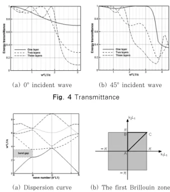
(a) 0° incident wave (b) 45° incident wave Fig. 4 Transmittance

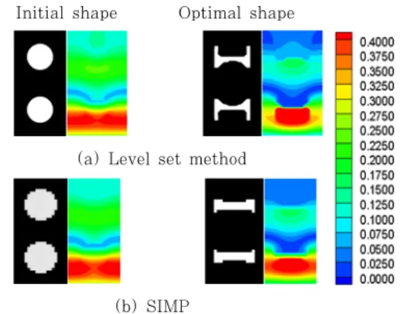
(a) Dispersion curve (b) The first Brillouin zone Fig. 5 Band gap for upper and lower half-infinites

Density Adiabatic bulk modulus

 and  _=1 =1

_ Scatter(inclusions) ^=1×10^-4 =1×10^-4

Outside of scatter _=1 =1

Table 1 Material properties

(a) One layer (b) Two layers (c) Three layers Fig. 3 Periodic sound barrier models

To decrease the performance measures, the design velocity for Hamilton Jacobi equation can be deter- mined as

n ( )

V ϕ J ξδ φ

φ

⎛∂ ⎞

= = −⎜⎝∂ + ⎟⎠ (38)

The Lagrangian multiplier ^ is determined from the Kuhn-Tucker optimality condition.

5. Numerical examples

5.1 Response analysis

This example is to show that the sound barrier model using the level set function is well working.

The scatterer in the sound barrier can be repre- sented by using the level set function as given in Fig. 3. Lets the material 1 is for the scatterer region, and material 2 is for the other region in sound barrier. Each material property is summ- arized in Table 1. The material interpolation is performed as

1 2

( ) H( ) {1 H( )}

ρ x =ρ φ ρ+ − φ ,

1 2

( ) H( ) {1 H( )}

β x =β φ β+ − φ (39)

For the two kinds of wave which propagate to the lower boundary of sound barrier with the angle of 0° and 45°, respectively, three kinds of layered sound barrier models as shown in Fig. 3 are tested.

Fig. 4 shows the results of the energy transmi- ttance for each incident angle. Fig. 5 shows the dispersion curves(Fig. 5(a)) of the infinite periodic domain corresponding to the layer with respect to the First Brillioun zone(Fig. 5(b)). Since there exists band gap between ^{ }2.5 and 3.5 along the A-B which corresponds to the incident wave of 0°

angle, the sound transmittance is reduced. However, for the case of 45° incident wave, three sound trans- mittances are not reduced on the same frequency region, since there is no band gap region. These facts show that the suggested methodology is working very well in the analysis for sound barrier.

5.2 Design sensitivity analysis

The purpose of this example is to verify the derived topological sensitivity expressions. The verification model is the sound barrier with one scatterer layer given in Fig. 3(a). The same model size and material properties are used with the example of section 4.1, and the 45° incident wave and frequency ^{ }2.33 are considered. In the level set method, the design variable is the level set function ^ at each position. To verify the accuracy of the developed

Evaluated

position Δ (a)E^r (∂E_r/∂φ δφ) (b) (b)/(a)×100 0˚ 8.079115E-06 8.073801E-06 100.0658 90^˚ -1.643022E-05 -1.641498E-05 100.0928 180˚ -2.169959E-05 -2.168293E-05 100.0768 270˚ 7.777268E-06 7.772083E-06 100.0667

Table 2 Verification of design sensitivity

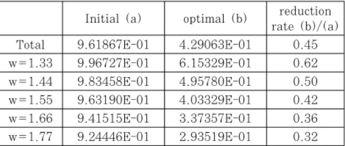
Initial shape Optimal shape

(a) Level set method

(b) SIMP

Fig. 6 Scatterer’s shape and acoustic pressure

Methods level set(a) SIMP(b) (a)/(b)

objectives 2.020958E-02 2.516300E-02 0.80 volume fraction 4.983686E-01 4.960320E-01 1.00

Table 3 Comparison of optimization results

(a) Optimization history (b) Energy transmittance Fig. 7 Optimization result for 45° incident wave analytical DSA methods using AVM, the variations

of the energy transmittance ^__ are compared with those from the forward finite diff- erence method (^∆__  ∆ _), where the amounts of design variation ^ and the design perturbation ^∆ are all 0.001. For sensitivity eval- uation, about the scatterer center, 0°, 90°, 180°, and 270° scatterer boundary positions are selected, and each angle is evaluated in the direction of counter clockwise from the right ends of the circular boundary. In Table 2, the analytical sensitivity results of AVM (b) show very good agreements with the finite difference results (a).

5.3 Shape optimization

5.3.1 Two layered periodic sound barrier

This example is for the comparison of level set based optimization with SIMP method about two scatters sound barrier model.

There is a volume constraint for scatter such that volume of ones is less than 50% of the original volume. Fig. 6 shows the optimization results of the level set based and the SIMP optimization for 0°

incident wave. As shown in Table 3, the level set based optimization results are smaller than the SIMP method by 20%. This is because the optimal shape of scatterer using level set result blocks the acoustic energy more effectively than the one using SIMP. Since the SIMP method has a limit to represent boundary distinctly as shown in Fig. 6(b), the level set based optimization is much reliable.

5.3.2 Three layered periodic sound barrier

This example is to show that our method is applicable to reduce the energy transmittance at a certain frequency region. The volume constraint is 50% of the original one, and the optimization is performed to minimize the energy transmittanc at 1.33^{  }1.77. Totally, 5 energy transmittances are picked up in this frequency region to evaluate performance measure, and the performance measure is given by a weighted summation of these values as

1

( ) ^N _rⁱ( )_{i i}

i

J φ E w

=

=

∑

where  is the energy transmattiance correspon- ding to i-th non dimensional frequecy ^, and ^ is the weight. Here, ^1 for all the cases ^{ }1,2,

…,5. The optimization results and history are shown in Fig. 7 for 45° incident waves. Tables 4 shows the optimization results at each frequency level for given incident waves. As shown these

Initial (a) optimal (b) reduction rate (b)/(a)

Total 9.61867E-01 4.29063E-01 0.45

w=1.33 9.96727E-01 6.15329E-01 0.62

w=1.44 9.83458E-01 4.95780E-01 0.50

w=1.55 9.63190E-01 4.03329E-01 0.42

w=1.66 9.41515E-01 3.37357E-01 0.36

w=1.77 9.24446E-01 2.93519E-01 0.32

Table 4 Minimization energy transmittance(45˚)

tables all energy transmittances at given frequency levels are decreased.

5. Conclusions

In this research, we performed level set based topological shape optimization for sound barrier with scatters. The derived shape design sensitivity is verified comparing with finite difference methods.

Using this sensitivity analysis, the level set based shape optimization was performed. By comparing these results with the SIMP based topology optimi- zation, it was proved that the developed method is well working. The level set method gives better results than SIMP since level set function improves the geometric exactness of scatterers. The objective function defined as energy transmittance guarantees optimum value since it is expressed as an energy quantity. In addition, it is possible to control energy transmittance at a certain frequency range where we want.

Acknowledgement

This research was supported by Basic Science Research Program through the National Research Foundation of Korea(NRF) funded by the Ministry of Education, Science and Technology(Grant Number 2010-18282). The support is gratefully ackno- wledged.

References

Abe, K., Nakayama, Y., Koro, K. (2010) Elastic wave pRopagation in Periodic Composite with Layer, JSCE Journal of Applied Mechanics, 13, pp.1041∼1048. (in Japanese)

Allaire, G., Jouve, F., Toader, A.M. (2004) Structural Optimization using Sensitivity Analysis and a Level-Set Method, Journal of Computational Physics, 194, pp.363∼393.

Bendsøe, M.P., Sigmund, O. (2003) Topology Optimization: Theory, Methods and Applications, Springer-Verlag, Berlin, p.370.

Håkansson, A., Sánchez-Dehesa, J., Sanchis, L.

(2004) Acoustic Lens Design by Genetic Algori- thms, Physical. Review B, 70, pp.214302.

He, L., CAO, C.Y., Osher, S. (2007) Incorporating Topological Derivatives into Shape Derivatives Based Level Set Methods, Journal of Computa- tional Physic, 225, pp.228∼242.

Qjan, Z.H., Jin, F., Li, F.M, Kishimoto, K. (2008) Complete Band Gaps in Two Dimensional Piezoe- lectric Phononic Crystals with {1-3} Connectivity Family, International Journal of Solids and Struc- tures, 45, pp.4748∼4755.

Sigmund, O, Jesen, J.S. (2003) Systematic Design of Phononic Band-Gap Materials and Structures by Topology Optimization, Philosophical Transactions : The Royal Society A, 361, pp.1001∼1019.

Vasseur, J.O., Djafari-Rouhani, B., Dobrzynski, L., Kushwaha, M.S., Halevi, P. (1994) Com- plete Acoustic Band Gaps in Periodic Fibre Rein- forced Composite Materials: the Carbon/Epoxy Composite and Some Metallic Systems, Journal of Physics: Condensed Matter, 6, pp.8759∼8770.

Yamada, T., Izui, K., Nishiwaki, S., Diaz, A-R., Nomura, T. (2010) Optimum Design of Photonic Band Gap Structures using Level Set-Based Topology Optimization Method, Proceeding of Confe- rence for Computational, Engieering Science, 15, pp.1085∼1088. (in Japanese)

요 지

본 논문에서는 레벨셋 방법을 이용하여, 소음을 차단하기 위한 음향 구조물의 형상 최적설계를 수행하였다. 형상 최적설 계의 목적은 특정한 각도와 각속도로 입사되는 입사파에 대해서 음향 투과율(acoustic transmittance)이 최소가 되도록 음향 결정의 형상(inclusion shape)을 결정하는 것이다. 음향 결정 구조에서는 음향이 흩어져 있는 결정 구조에 의해서 굴절되기 때문에 결정 모양을 조정함으로써, 음향 거동을 제어할 수 있다. 본 연구에서는 음향 구조물로 결정이 수평방향으로는 주기 적으로 무한히 분포하고 수직방향으로는 유한한 층간 구조를 가지고 있는 소음 방어벽(Noise barrier)을 고려한다. 주기적 구조물을 고려하기 때문에 결정의 좌와 우에 Bloch 이론을 적용해 주기적 경계조건을 부과하였고, 소음 방어벽 위와 아래에 는 임피던스 행렬(impedance matrix)를 이용하여, 무한 균질 영역과 소음 방어벽 사이의 음파 투과를 모사하였다. 결정의 위 상과 형상변화를 묘사하기 위해서 레벨셋 방법(level set method)을 사용하였다. 레벨셋 방법에서는 초기 영역을 고정시킨 상태에서, 레벨셋으로 표현되는 임시적 경계(implicit moving boundary)를 변화시킴으로써 복잡한 형상을 다룰 수 있다. 몇 몇 수치적 예제를 통해, 제시된 방법의 적용성을 검증하였다.

핵심용어 : 위상 및 형상 최적설계, 레벨셋 방법, 소음벽 거동, Bloch 이론, 음향파 투과율, 보조변수 방법