Thermal Image Mosaicking Using Optimized FAST Algorithm

(1)

https://doi.org/10.7848/ksgpc.2017.35.1.41

Thermal Image Mosaicking Using Optimized FAST Algorithm

Nguyen, Truong Linh

¹⁾

ㆍHan, Dong Yeob

²⁾

Abstract

A thermal camera is used to obtain thermal information of a certain area. However, it is difficult to depict all the information of an area in an individual thermal image. To form a high-resolution panoramic thermal image, we propose an optimized FAST (feature from accelerated segment test) algorithm to combine two or more images of the same scene. The FAST is an accurate and fast algorithm that yields good positional accuracy and high point reliability; however, the major limitation of a FAST detector is that multiple features are detected adjacent to one another and the interest points cannot be obtained under no significant difference in thermal images. Our proposed algorithm not only detects the features in thermal images easily, but also takes advantage of the speed of the FAST algorithm. Quantitative evaluation shows that our proposed technique is time-efficient and accurate. Finally, we create a mosaic of the video to analyze a comprehensive view of the scene.

Keywords : Image Stitching, Image Feature Detection, Thermal Image, Optimized Fast Algorithm

Original article

Received 2017. 01. 16, Revised 2017. 01. 31, Accepted 2017. 02. 15

1) Member, Dept. of Civil and Environmental Engineering, Chonnam National University (E-mail: [email protected])

2) Corresponding Author, Member, Dept. of Marine and Civil Engineering, Chonnam National University (E-mail: [email protected])

This is an Open Access article distributed under the terms of the Creative Commons Attribution Non-Commercial License (http://

creativecommons.org/licenses/by-nc/3.0) which permits unrestricted non-commercial use, distribution, and reproduction in any medium,

1. Introduction

Image mosaicking is a technique in which several overlapp- ing images are combined to form a panoramic image of high resolution. Recent development of mobile imaging leads to research interest in mosaic image creation. Depending on the tile dataset and the imposed constraints for positioning the deformations, various mosaics can be created for an image.

Thermal video mosaicking allows the creation of a large field of view using a thermal camera, and in some specific cases, it is used by managers to support decision making from an evaluation of the temperature distribution.

Image stitching techniques can be categorized into two general approaches: direct and feature based techniques. In the direct technique, pixel-to-pixel dissimilarity is minimized to perform image stitching. Meanwhile, in the feature-based technique, a set of features is extracted and then matched with each other (Arya, 2015). The development of feature detection techniques for image mosaicking is an important

research subject in the field of computer vision (Bheda et al., 2014). There are several feature detection techniques, which include SIFT (scale-invariant feature transform) (Lowe,2004;

Alhwarin et al., 2008; Kai et al., 2012), FAST (Adel et al., 2014), SURF (speeded-up robust feature) (Bay et al., 2008;

Adel et al., 2014; Pravenaa and Mennaka, 2016), Harris (Jain et al., 2012), PCA – SIFT (Ke and Sukthankar, 2004), and ORB (Rublee et al., 2011) techniques. The SIFT technique is very robust; however, the computation time makes it less feasible. The Harris corner is not invariant to scale changes and needs to set a threshold value. Many redundant corners can be occurred or effective corners can be lost by uncertain threshold selection. The SURF is a fast and robust algorithm;

however, it is poor at handling viewpoint and illumination changes. The FAST algorithm can detect the interest points for real-time applications; however, the major limitation of FAST is that multiple features are detected adjacent to one another.

Several studies on image mosaicking have been carried

(2)

out. A study conducted by Manmohan Sharma (2014) at the IIITA Campus (Indian Institute of Information Technology, Allahabad) included steps such as selecting the control points, image writing, and blending on the images taken with the help of a digital camera (Sharma, 2014). It enables the user to obtain a very wide-angle image without using any expensive wide-angle camera. A new compact large FOV (Field Of View) multi-camera system is introduced (Lu et al., 2016). The camera has seven small complementary metal-oxide-semiconductor sensor modules, which can obtain seven images in a single shot at the rate of 13 frames per second. The actual luminance of the objects was used to blend the images to create panoramas, so that the final image reﬂects the objective luminance accurately. A method for the construction of a mosaic from video sequences obtained by rotating the camera was presented in study of Hoseini and Jafari (2011). The distinctive features are first detected and matched using a localized scene coherence method, and then, the mapping function parameters are estimated for feature matching. The frames are mapped to the surface of the middle frame using the obtained transformations, and finally, the warped frames are combined (Hoseini and Jafari, 2011).

Several works in the literature have already improved the algorithm with an aim to reduce the computation time of SIFT. Kai et al. (2012) used the original SIFT algorithm to extract numerous matching points and the precise matching points were selected using the maximum of minimum distance cluster algorithm. This optimized SIFT can avoid noise and structurally unrelated matching points, and thus

improve the accuracy of image matching. Alhwarin et al.

(2008) improved the SIFT algorithm by dividing the features extracted from both the test and the model object image into several sub-collections before they are matched. In addition, from the different frequency domains, the features are divided into several sub-collections by considering the features arising from different octaves. Compared to the original SIFT algorithm, 40% reduction in the processing time for matching the stereo images was achieved.

This paper presents a mosaicking technique for thermal images that have relatively small number of feature. We propose an optimized FAST algorithm that takes advantage of the quickness of the FAST algorithm, but overcomes its disadvantages.

2. Image Mosaicking

2.1 The steps of image mosaicking

Image mosaicking is an important technique in the field of computer vision, image processing, and panoramic image creation. Image mosaicking involves the stitching of multiple correlated images to generate a single large seamless image (Bheda et al., 2014). It requires an understanding of the geometric relationships between images. The geometric relations are affine transformations that relate the coordinate systems of different images (Sharma, 2014). Image stitching can be divided into three main processes: calibration, image registration, and blending. The goal of camera calibration is to produce an estimate of the extrinsic and intrinsic camera parameters. During image registration, multiple images are Fig. 1. Steps of image mosaicking

Collecting different images that have overlapping regions

Calculating the transformation matrix between the two images

Obtaining the final image in panoramic view

Blending the stitched border of the image so that the image is seamless

Stitching up the images using

the transformation

matrix

(3)

compared to obtain the translations that can be used for the alignment of images. After registration, these images are merged to form a single image. Then, image blending technique will be used to modify the gray levels of image in the vicinity of a boundary to obtain a smooth transition between images. The overall process of image mosaicking is shown in Fig. 1.

2.2 Determination of the orientation of the image

2.2.1 DLT (Direct Linear Transformation)

DLT describes a direct connection between the 3D and image coordinates (Molnar, 2010). This method is based on the collinearity equations, extended by an affine transformation of the image coordinates. It does not require the image coordinate system to be fixed with the camera. The transformation equation of the DLT is given by Eq. (1):

1 2 3 4

9 10 11

5 6 7 8

9 10 11

1 1 L X L Y L Z L x L X L Y L Z

L X L Y L Z L y L X L Y L Z

 + + + 

=   + + +  

 + + + 

=   + + +  

(1)

where L

i

: DLT parameters, x, y: image coordinates, X, Y, Z: 3D coordinates.

Determination of the 11 DLT parameters requires a minimum of 6 reference points. The calculation is processed in two steps: first, the DLT parameters are estimated using the control points for each image, and the unknown points are then calculated if they appear on more than two oriented images. The least squares method, with some modifications,

is used for the adjustment.

2.2.2 BA (Bundle Adjustment)

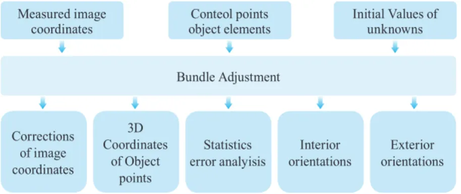
Fig. 2 shows the principle data ﬂow for a BA process. The input data for the BA are typically photogrammetry image coordinates generated by manual or automatic (digital) image measuring systems. Additional information in the object space can also be taken into account. They provide the definition of an absolute scale and the position and orientation of the object coordinate system. This information is entered into the system as, for example, reference point files or additional observations. In order to linearize the functional model, approximate values must be generated.

The principal results of the BA are the estimated 3D coordinates of the object points. In addition, the exterior orientation parameters of all the images are estimated.

The interior orientation parameters are estimated if the cameras are calibrated simultaneously within the adjustment (Luhmann et al., 2006).

The collinearity equations (Eq. (2)) are a mathematical model for the bundle block adjustment. The mathematical model consists of both functional and stochastic models (Lee and Yu, 2009).

( ) ( ) ( )

11 0 21 0 31 0

' ' ' '

0

13 0 23 0 33 0

12 0 22 0 32 0

' ' ' '

0

13 0 23 0 33 0

r X X r Y Y r Z Z

x x z x

r X X r Y Y r Z Z r X X r Y Y r Z Z

y y z y

r X X r Y Y r Z Z

− + − + −

= + + ∆

− + − + −

= + + ∆

− + − + −

(2)

The structure of these equations allows the direct formulat-

Fig. 2. Data ﬂow for the BA process Corrections

of image coordinates

Coordinates 3D of Object

points

Statistics

error analyisis Interior

orientations Exterior orientations Bundle Adjustment

Conteol points

object elements Initial Values of unknowns Measured image

coordinates

(4)

ion of primarily observed values (image coordin-ates) as functions of all unknown parameters in the photogramme- tric imaging process. The collinearity equations, linearized at approximate values, can be used directly as observation equations for a least-squares adjustment according to the Gauss-Markov model.

2.3 Space intersection

Space forward intersection is commonly used to determine the ground coordinates X, Y, and Z of points that appear in the overlapping areas of two or more images based on known interior and exterior orientation parameters. The collinearity condition, which states that the corresponding light rays from the two exposure stations pass through the corresponding image points on the two images and intersect at the same ground point, is enforced. Fig. 3 illustrates the principle of forward intersection (Jia et al., 2010), where P is an arbitrary point on the ground, O1 and O2 indicate the camera station, and p1 and p2 are the corresponding image points of P.

Space forward intersection techniques assume that the exterior orientation parameters associated with the images are known. Using the collinearity equations, the exterior orientation parameters along with the image coordinate measurements of point P on Image 1 and Image 2 are input to compute the X

P

, Y

P

, and Z

P

coordinates of the ground point P.

2.4 RANSAC (RANdom SAmple Consensus) algorithm

The RANSAC algorithm proposed by Fischler and Bolles, (1981) is a general parameter estimation approach designed to cope with a large proportion of outliers in the input data. The RANSAC algorithm has four steps:

(1) Randomly select the minimum number of points required to determine the model parameters

(2) Solve for the parameters of the model

(3) Determine the number of points from the set of all points that fit with a predefined tolerance

(4) If the fraction of the number of inliers over the total number of points in the set exceeds a predefined threshold t, re-estimate the model parameters using all the identified inliers and terminate the process (5) Otherwise, repeat steps 1 through 4

The number of iterations is chosen high enough to ensure that the probability that at least one of the sets of random samples does not include an outlier.

2.5 Blending

Once we have registered all the input images with respect to each other, we need to decide how to produce the final stitched image. First, a compositing surface, which is ﬂat and cylindrical, is chosen. Next, it is decided how to blend them to create the panorama.

For stitching fewer images, a natural approach is to select one of the images as the reference and then warping all the images according to the reference coordinate system. The colors are adjusted to compensate for the exposure differences between images. The images are blended together and the seam line is adjusted to minimize the visibility of seams between images (Shashank et al., 2014).

3. The Optimized FAST Descriptor

Before image registration and alignment, the mathematical relationship between the pixels coordinates of one image with respect to the others need to be established (Pravenaa and Mennaka, 2016). Both direct and feature based techniques are considered for image stitching.

In the direct technique, all the pixel intensities of the image

Fig. 3. Space intersection

(5)

are compared with each other. In this technique, each pixel is compared with each other, and therefore it is a very complex technique. The main advantage of the direct method is that they make optimal use of the information available in the image alignment. They measure the contribution of every pixel in the image. The main limitation of this technique is a limited range of convergence between one another (Adel et al., 2014).

In feature-based techniques, all the feature points in an image pair are compared with that of every feature in another image, using local descriptors. The different steps required for image stitching based on feature-based techniques are feature extraction, registration, and blending. Feature-based methods begin by establishing correspondences between points, lines, edges, corners, or other shapes (Adel et al., 2014). The uniqueness of the robust detectors incorporates invariance to the noisy image, scale invariance, translation invariance, and rotation transformations. There are several feature detection techniques, such as SIFT, SURF, and FAST (Rosten and Drummond, 2006).

3.1 SIFT

The SIFT operator is one of the most frequently used technique for region detection. It was first conceived by Lowe, (2004) and is currently employed for various applications (Lingua et al., 2009). The SIFT algorithm for image feature generation is invariant to image translation, scaling, and rotation and is partially invariant to illumination changes and affine projection (Alhwarin et al., 2008). SIFT can be used to identify similar objects in other images. When checking for an image match, two sets of key-point descriptors are given as input to the NNS (Nearest Neighbor Search) problem and closely matching key-point descriptors are produced.

The SIFT algorithm consists of four stages (Aghdasi et al., 2009; Kai et al., 2012; Adel et al., 2014; Bheda et al., 2014).

Scale-space local extrema detection, Key-point localization, Orientation assignment, Key-point descriptor. Though it is comparatively slow, the SIFT algorithm is a robust algorithm for image comparison. The running time of a SIFT algorithm is high as it takes more time to compare two images.

3.2 SURF

SURF is an algorithm developed for local, similarity

invariant representation and comparison (Bay et al., 2008). In addition, Bay demonstrated that the SURF detector is several times faster than SIFT and more robust against different image transformations (Besbes et al., 2015). The SURF algorithm is performed in three main steps (Adel et al., 2014; Pravenaa and Mennaka, 2016). Detection, Description, Matching. The main advantage of the SURF approach lies in its fast computation, enabling real-time applications such as tracking and object recognition. It improves upon the speed of the SIFT detection process by giving priority to the quality of the detected points. It gives more focus on speeding-up the matching step.

3.3 Optimization of FAST algorithm

The FAST technique identifies interest points in an image (Adel et al., 2014). The pixel A is recognized as a FAST corner if the neighborhood around pixel A has sufficient pixels, which are in a gray that is different from the pixel A.

The FAST detector compares the pixels only on a circle of fixed radius around a point. A point is classified as a corner only if a large set of pixels that are significantly brighter or darker than the central point can be found in a circle of fixed radius around the point. As shown in Fig. 4, the FAST algorithm considers a circle of 16 pixels around the corner candidate p. An interesting point is indicated when all the pixels in a set of n contiguous pixels in the circle are brighter than the candidate pixel I

^p

plus a threshold t, or all the pixels are darker than I

^p

≤ t shown in Eq. (3). The corner detector should satisfy the following criteria (Arya, 2015).

(1) The detected positions should be consistent, insensitive to the variation of noise, and they should not move when multiple images of the same scene are acquired.

(2) Accuracy: The corners should be detected as close as possible to the correct positions.

(3) Speed: The corner detector should be fast enough.

FAST is an accurate and fast algorithm that yields good positional accuracy and high point reliability.

x p

I − I > t (3)

(6)

The two major limitations of the FAST detector are that multiple features are detected adjacent to one another and that the features cannot be detected if the image has no significant difference in gray-scale values. It means that, we do not obtain the pixel p, which satisfies the condition of being brighter or darker than a circle of 9 or 12 pixels. In other words, p satisfying the above equation does not exist.

To overcome this limitation, the image data need to be pre- processed.

First, by considering the overall gray value of the input images, all the positions where there are significant differences in gray values are found. The region that includes 16 pixels around the pixel that satisfies the conditions of the algorithm is obtained like that shown in Fig. 4. Second, using the FAST algorithm, the position in the image where no pixels have been found is chosen and compared with 16 pixels surrounding it, to decrease the cost time. The optimized FAST

Fig. 4. FAST corner detection

algorithm used in this paper is summarized in Fig. 5. With the input image, the portions that have significant difference in gray value will be found, that portions are saved as the point p (h, v). Then, the region include 16 pixels around the position p (h, v) will be obtained. Set the value for other pixels to find the difference from the region of 16 pixels. From that, all new values are saved to new matrix M (1: h, 1: v). From now, the input data of algorithm is not original input image which was processed, the input data for algorithm is matrix M.

4. Experiment

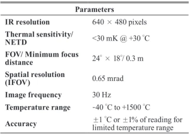
The thermal camera (FLIR SC660 shown in Fig. 6) provides a combination of infrared and visible spectrum images that have superior quality and temperature measurement accuracy, and features a contrast optimizer, laser pointer, voice annotation, and a host of other advanced features. It can measure the temperature by taking a thermal image, sequence video, or video. The FLIR SC660 has a high-resolution pixel detector of 640×480 pixels having a high accuracy. Table 1 shows the technical specifications of FLIR SC660 Flir-Systems, 2008().

Input images

Output feature points of images

1 2

3 4 5 6 7 8 10 9

11 12 13 14 15 16 17

for i = 1 to h (h, v is size of image) for j =1 to v

find the portions that have significant difference in gray value

save the point p (h, v)

obtain the region including 16 pixels around the position p (h, v)

set the value for other pixels to find the difference from the region of 16 pixels

save all new values to a new matrix M (1:h,1:v) next j

next i

do FAST algorithm on M:

choose the pixel p in the region of 16 pixels compare p (h, v) with 16 pixels around in matrix M if p is max or min

choose p as the candidate point save p

end if

Fig. 5. Procedure for the algorithm

Parameters

IR resolution 640 × 480 pixels Thermal sensitivity/

NETD <30 mK @ +30 °C

FOV/ Minimum focus

distance 24° × 18°/ 0.3 m

Spatial resolution

(IFOV) 0.65 mrad

Image frequency 30 Hz

Temperature range -40 °C to +1500 °C

Accuracy ±1 °C or ±1% of reading for

limited temperature range

Table 1. Thermal camera SC660 speciﬁcation

(7)

The data shown in Fig. 7 was obtained at Chonnam National University by using the thermal camera FLIR SC660. The data used in this study is a sequence video. The video was obtained by the camera at Buildings 2 and 3 of Chonnam National University, from right to left, towards the vertical surfaces of the building. Before obtaining the data, some camera parameters need to be set up. Some basic parameters are shown in Table 2.

Table 2. Setup parameters for thermal camera before obtaining video

Parameters

Object Emissivity (0 to 1) 0.95

Distance (m) 20

Atmosphere Atmospheric Temp (°C) 7 Relative Humidity (%) 72 External Optics Temperature (°C) 10 Transmission (0 to 1) 1 Acquisition date 2015-12-09

To obtain the control points on the walls of the building, a total station was used to measure the points. The points were evenly distributed on the walls of Buildings 2 and 3. In addition, we obtained sufficient control points in each image and in the overlapping areas of the photos. Specifically, at least 6 control points for each image and 3 common points in the overlapping region.

5. Result and Discussion

5.1 Comparison of the DLT and BA results The data include 10 images captured by the thermal camera FLIR SC660. From each image, two positions were chosen for the comparison; thus, 20 positions were chosen. After calculating the 6DOF using the DLT and BA methods, the position accuracy in Table 4 was evaluated using the camera’s position and rotation parameters in Table 3. Finally, the root mean square error was calculated. For the DLT method, the errors dx and dy are 5.82 and 6.26, respectively. For the BA method, dx and dy are 1.37 and 0.65, respectively. From the comparison of the results obtained by the DLT and BA methods, it can be observed that the values obtained using both the methods show a fair accuracy. However, the results obtained by the BA method are more precise. The BA method provides precise and easily interpretable results, because it uses accurate statistical error models and supports a sound, well-developed quality control methodology.

5.2 Discrepancy

After obtaining the 6EOP results, we considered the discrepancy between the corresponding points of one image and the overlapping image. The trend of inconsistency errors was determined in this way.

Fig. 6. Thermal camera FLIR SC660

Fig. 7. Thermal image obtained by thermal camera SC660

(8)

Image Omega (°) Phi (°) Kappa (°) X (m) Y (m) Z (m)

1 112.476 -74.367 -328.678 40.036 -59.065 22.292

2 112.556 -74.423 29.755 38.146 -52.261 23.308

3 114.276 -72.990 29.451 33.517 -33.952 19.325

4 109.784 -73.269 23.641 32.346 -28.453 17.064

5 115.417 -72.701 28.597 30.801 -23.243 18.966

6 114.525 -71.355 25.757 27.184 -11.522 20.168

7 110.909 -70.807 20.194 21.556 5.6230 21.105

8 109.316 -69.353 17.517 19.954 10.544 21.329

9 119.716 -68.130 25.143 15.031 23.524 19.418

10 118.788 -63.626 23.014 14.269 26.802 17.999

Images Points and

Observed image points

(pixel)

Calculated by

DLT (pixel) Calculated by

BA (pixel) Accuracy of DLT

(pixel) Accuracy of BA (pixel)

x y x-DLT y-DLT x-BA y-BA dx-DLT dy-DLT dx-BA dy-BA

1 5 361 329 360.88 330.24 361.08 329.01 0.12 -1.24 -0.08 -0.01

1 8 190 335 187.29 335.61 189.98 335.42 2.71 -0.61 0.02 -0.42

2 5 484 363 483.84 363.42 484.74 362.51 0.16 -0.42 -0.74 0.49

2 8 314 375 312.59 374.25 314.96 374.06 1.41 0.75 -0.96 0.94

3 5 492 254 491.53 253.27 490.80 254.18 0.47 0.73 1.2 -0.18

3 8 373 263 373.00 262.10 373.71 261.56 0 0.90 -0.71 1.44

4 5 493 368 492.62 370.02 492.28 367.46 0.38 -2.02 0.72 0.54

4 8 201 237 203.11 236.93 201.27 236.90 -2.11 0.07 -0.27 0.10

5 5 296 296 294.26 294.39 295.46 296.06 1.74 1.61 0.54 -0.06

5 8 184 389 190.61 384.21 183.77 388.01 -6.61 4.79 0.23 0.99

6 5 424 345 416.69 342.50 423.77 345.66 7.31 2.50 0.23 -0.66

6 8 260 324 275.18 345.26 260.33 323.82 -15.18 -21.26 -0.33 0.18

7 5 423 262 429.75 248.81 422.81 261.74 -6.75 13.19 0.19 0.26

7 8 319 215 310.85 212.26 319.06 214.84 8.15 2.74 -0.06 0.16

8 5 434 217 430.05 221.65 434.01 217.13 3.95 -4.65 -0.01 -0.13

8 8 435 434 436.97 427.04 435.03 433.64 -1.97 6.96 -0.03 0.36

9 5 461 343 450.48 342.22 458.31 343.62 10.52 0.78 2.69 -0.62

9 8 289 265 288.93 265.07 293.01 266.24 0.07 -0.07 -4.01 -1.24

10 5 386 204 392.91 204.1 388.75 203.61 -6.91 -0.1 -2.75 0.39

10 8 150 213 152.97 213.1 150.39 213.71 -2.97 -0.1 -0.39 -0.71

RMSE 5.82 6.26 1.37 0.65

Table 3. Exterior orientation parameters of the images from the BA method

Table 4. Accuracy of DLT and BA results

(9)

determine the trend of inconsistency errors we considered two cases. Fig. 8 shows the check points in the horizontal direction, while Fig. 10 shows in the vertical direction. In the horizontal case, 22 positions were chosen from the left through the center and to the right. In the vertical case, 16 positions were chosen from the top through the center and to the bottom. As seen in Fig. 9, for the points from 4 to 12, the error is less than 0.2. However, the other points (1 to 3 and 13 to 22) under the marginal portion of the overlap show a low accuracy, with the error greater than 0.23. In particular, the points from 18 to 22 have a significantly low accuracy.

Similar to the first case, in Fig. 11, the points from 4 to 12 have a high accuracy; however, point 1 and the points from 13 to 16 have a low accuracy. It shows that the position in the central part of the overlap between the two images has a consistently high accuracy, and the marginal portion has a low accuracy. It can be inferred that the greater the distance from the center, the lower will be the accuracy.

5.3 Extraction results

To verify whether the optimization FAST algorithm is feasible, the paper compares the classical SIFT algorithm and SURF algorithm with the FAST detection algorithm.

Two groups of images shown in Fig. 12 were considered for validation. The first set of pictures was taken from the thermal video (with a size 640×480 and a depth of 8 bit);

two images of this group were overlapped. The second set of pictures has a size 225×225 with a depth of 24 bit; two images of this group are rotated 90 degrees, and all the images are in jpg format.

Figs. 9 and 11 describe the trend discrepancy between corresponding points of two overlapping images. To

Fig. 8. Positions chosen in the overlapping images for checking accuracy in the horizontal direction

Fig. 10. Positions chosen in the overlapping images for checking accuracy in the vertical direction

(a) Fig. 9. Discrepancy between corresponding points in the

horizontal direction

Fig. 11. Discrepancy between corresponding points in the

vertical direction

(10)

Fig. 13 shows the results of the image matching based on FAST and optimized FAST algorithms of the two sets. From Fig. 13(a), which shows the FAST algorithm matching result, it can be seen that only 2 points were extracted, because the gray value does not have any significant difference.

However, when the optimized FAST was used, more points were extracted, as shown in Fig. 13(b). Similarly, for the second set, shown in Figs. 13(c) and 13(d), we can see that the optimized FAST algorithm has more points than the FAST algorithm. The details are listed in Table 5.

(b)

Fig. 12. Two sets of original images. a) 640×640 and 8 bit; b) 225×225 and 24 bit

(a)

(b)

(c)

(d)

Fig. 13. The results of image matching based on FAST and optimized FAST algorithms: (a) FAST algorithm of 640×480 image; (b) Optimized FAST algorithm of 640×480 image; (c) FAST algorithm of 225×225 image;

(d) Optimized FAST algorithm of 225×225 image

Table 5. The results of different algorithms

Algorithm

Stereo image 1

640 × 480 (8 bit) Stereo image 2 225 × 225 (24 bit) Number

inliers of

Matching Time(s)

Number inliers of

Matching Time(s)

SIFT 367 1.502 12 0.752

SURF 36 1.281 92 0.263

FAST 2 0.359 92 0.146

Optimized

FAST 49 0.366 103 0.160

(11)

By comparing the data of Table 5, we can see that the time consumption for the SIFT algorithm is much higher than those of SURF and FAST algorithms (Refer to the Fig. 14).

The time taken for the SIFT algorithm for Stereo 1 is 1.502 s, while those for the SURF and FAST algorithms are just 1.281 s and 0.359 s, respectively. Similarly, for Stereo 2, the time for SIFT is 0.752 s, which is thrice that of SURF and several times that of FAST. In both cases, the FAST algorithm is the fastest, (0.359 s and 0.146 s). This is a good technique; however, the major limitation is that it cannot detect the features when the images have no significant difference in gray values, like Stereo 1. Thus, the number of inliers is only 2. After we optimized the FAST, the number of features became 49, while the time consumption was similar. In the second case, the optimized FAST can detect more number of features than the FAST algorithm, thereby ensuring accuracy. In this case, the FAST detected 92 features, while the optimized FAST detected 103 features, thus proving the effectiveness of data processing before applying the FAST algorithm.

5.4 Thermal mosaicking

Fig. 15 shows all the images (10 images) in the mosaicking process. Fig. 16 shows the resulting image after mosaicking and referenced by the heat color. All the images in the thermal video were stitched. From this image, some temperature information about the building will be obtained, as the light- red color indicates areas that have a temperature of 11–15 °C.

The rooms, which have a higher temperature than the other areas, were part of the laboratory in which an experiment was being conducted. Some windows, which have a temperature around 9 °C, show that there was a heat leakage. In winter, all the rooms have heaters, causing the inside temperature to

be higher than the outside temperature. The windows have an inability to retain heat, which is the cause of heat leakage.

6. Conclusion

This paper proposed an improvement of the feature extraction algorithm based on the FAST algorithm. By finding positions that have significant differences in gray values in a region of 16 pixels around the position, and by assigning a new value for the other pixels and comparing those pixels with others, the optimized FAST algorithm increases the number of feature points that are detected. The universal applicability of the optimized FAST algorithm is verified by two sets of images, especially with the thermal images. It shows that the optimized FAST algorithm overcame the disadvantages of the FAST algorithm. In addition, the paper has presented the steps required to mosaic two images together by using the optimized FAST algorithm to detect the feature points. The results of mosaicking show a comprehensive view of two buildings in Chonnam National University, obtained from thermal images. With this result, it is easier to cover the surface temperature distribution of a building, enabling managers to have a better overview of the object zone and take correct decisions.

However, the time cost of the optimized algorithm is Fig. 16. Thermal image after mosaicking

Fig. 15. All the images from the thermal video

Fig. 14. Comparison of cost time between algorithms

(12)

greater than the FAST algorithm and the multiple features are detected still adjacent to one another. Therefore, the future research should focus on reducing the time and the feature adjacent.

Acknowledgment

This research was supported by a grant (16RDRP-B076564 -03) from Regional Development Research Program funded by Ministry of Land, Infrastructure and Transport of Korean government.

References

Adel, E., Elmogy, M., and Elbakry, H. (2014), Image stitching based on feature extraction techniques - A survey, International Journal of Computer Applications, Vol. 99, No. 6, pp. 1-8.

Aghdasi, H.S., Bisadi, P., Moghaddam, M.E., and Abbaspour, M. (2009), High-resolution images with minimum energy dissipation and maximum field-of-view in camera-based wireless multimedia sensor networks, Sensors, Vol. 9, No.

8, pp. 6385-6410.

Alhwarin, F., Wang, C., Durrant, D.R., and Graser, A.

(2008), Improved SIFT–features matching for object recognition, Proceedings of BCS International Academic Conference 2008 – Vision of Computer Science, BCS, 22- 24 September, London, UK, pp. 179-190.

Arya, S. (2015), A review on image stitching and its different methods, International Journal of Advanced Research in Computer Science and Software Engineering, Vol. 5, No.

5, pp. 299-303.

Bay, H., Tuytelaars, T., and Gool, L.V. (2008), Speeded-up robust features (SURF), Computer Vision and Image Understanding, Vol. 110, No. 3, pp. 346-359.

Besbes, B., Rogozan, A., Rus, A.M., Bensrhair, A., and Broggi, A. (2015), Pedestrian detection in far-infrared daytime images using a hierarchical codebook of SURF, Sensors, Vol. 15, No. 4, pp. 8570-8594.

Bheda, D., Joshi, M., and Agrawal, V. (2014), A study on features extraction techniques for images mosaicing, International Journal of Innovative Research in Computer and Communication Engineering, Vol. 2, No. 3, pp. 3432-

3437.

Fischler, M.A. and Bolles, R.C. (1981), Random sample consensus: A paradigm for model fitting with applications to image analysis and automated cartography, Communi- cations of the ACM, Vol. 24, No. 6, pp. 381-395.

Flir-Systems, (2008), FLIR SC660 R&D Infrared camera system, FLIR Systems, Hong Kong, http://www.ﬂir.com/

uploadedFiles/Thermography_APAC/Products/Product_

Literture/SC660_Datasheet%20APAC(1).pdf (last date accessed 16 January 2017).

Hoseini, S.A. and Jafari, S. (2011), An automated method for mosaicking of video frames with projective constraint, International Journal of Science and Advanced Technolo- gy, Vol. 1, pp. 112-116.

Jain, D.K., Saxena, G., and Singh, V.K. (2012), Image mosaicing using corner techniques, Proceedings of In- ternational Conference on Communication Systems and Network Technologies, IEEE, 11-13 May, Washington, USA, Vol. 12, pp. 79-84.

Jia, G., Wang, X., Wang, H.B., and Zhang, Z. (2010), Accuracy analysis of space three line array photogrammetry based on forward intersection, Proceedings of 2010 3rd International Conference on Advanced Computer Theory and Engineering, ICACTE, 20-22 Aug, Chengdu, China, Vol. 1, pp. 391-395.

Kai, W., Bo, C., and Long, T. (2012), An improved SIFT feature matching algorithm based on maximizing minimum distance cluster, Proceedings of 2011 Internat- ional Conference on Computer Science and Information Technology, ICCSIT, 10-12 June, Chengdu, China, vol. 51, pp. 255-259.

Ke, Y. and Sukthankar, R. (2004), PCA-SIFT: A more distinctive representation for local image descriptors, Proceedings of the 2004 IEEE Computer Society Con- ference on Computer Vision and Pattern Recognition, IEEE, 27 June - 2 July, Washington DC, USA, Vol. 2, pp.

506-513.

Lee, W. and Yu, K. (2009), Bundle block adjustment with 3D natural cubic splines, Sensors, Vol. 9, No. 12, pp. 9629-9665.

Lingua, A., Marenchino, D., and Nex, F. (2009), Performance

analysis of the SIFT operator for automatic feature

extraction and matching in photogrammetric applications,

(13)

Sensors, Vol. 9, No. 5, pp. 3745-3766.

Lowe, D.G. (2004), Distinctive image features from scale- invariant keypoints, International Journal of Computer Vision, Vol. 60, No. 2, pp. 91-110.

Lu, Y., Wang, K., and Fan, G. (2016), Photometric calibration and image stitching for a large field of view multi-camera system, Sensors, Vol. 16, No. 4, 516 p.

Luhmann, T., Robson, S., Kyle, S., and Harley, I. (2006), Close Range Photogrammetry Principles, Methods and Applications, Whittles Publishing, Scotland, UK.

Molnar, B. (2010), Direct linear transformation based photo- grammetry software on the web, International Archives of Photogrammetry, Remote Sensing, and Spatial In- formation Sciences, ISPRS, 21-24 June, Newcastle, UK, Vol. XXXVIII, Part 5, pp. 462-465.

Pravenaa, S. and Mennaka, R. (2016), A methodical review on image stitching and video stitching techniques, In- ternational Journal of Applied Engineering Research, Vol.

11, No. 5, pp. 3442-3448.

Rosten, E. and Drummond, T. (2006), Machine learning for high-speed corner detection, Proceedings of European Conference on Computer Vision, ECCV, 7-13 May, Graz, Austria, pp. 430-443.

Rublee, E., Rabaud, V., Konolige, K., and Bradski, G.

(2011), ORB: An efficient alternative to SIFT or SURF, Proceedings of 2011 International Conference on Computer Vision, IEEE, 6-13 November, Barcelona, Spain, pp. 2564-2571.

Sharma, M. (2014), Image mosaicing and producing a panoramic visibility, International Journal on Recent and Innovation Trends Computing and Communation, Vol. 2, No. 2, pp. 198-201.