A Study on the Spatial Distribution Patterns of Urban Green Spaces Using Local Spatial Autocorrelation Statistics
21
0
0
전체 글
(2) 김윤기. Other researchers also tried to confirm the. they could not identify which area is a hotspot and. relationship between the distribution patterns of. which area is a coldspot.. green spaces and the health of citizens (Georgi et. Many scholars use the Global Moran’s index to. al. 2010; Shackleton et al. 2015). In particular,. analyze the global spatial distribution pattern of a. Albert et al. (2017) examined the association between. particular phenomenon. The index shows whether. the distribution patterns of green spaces in cities. a particular phenomenon is distributed in a. and the birth outcome. Their findings show that. specific order or randomly in space. The Moran's. the distribution patterns of green spaces are. index has a value between -1 and 1 (Tiefelsdorf. closely related to the birth outcome. Some scholars. 2002). A value of 1 signifies perfect positive spatial. have focused much attention on the spatial. autocorrelation, a value of –1 indicates perfect. disparities of the green space distribution (Wen et. negative spatial autocorrelation, and a value of 0. al. 2013; Hoffimann et al. 2017; Wüstemann et al.. means perfect spatial randomness (Dalposso et al.. 2017). In particular, Wen et al. (2013) attempted to. 2013). We can also use this index to determine. identify what factors influenced access to green. whether similar values are clustered or scattered. spaces and parks. Their research results show that. in space. To accurately investigate the spatial. poverty levels affected negatively on access to. distribution patterns of green spaces in cities,. green spaces.. scholars must consider not only the global. Most previous studies have used satellite or. dimension but also the local dimension. Numerous. UAV images to identify urban green space distri-. researchers today use local spatial autocorrelation. bution patterns. In other words, many researchers. statistics, such as the Local Moran’s index, the. used vegetation indices such as NDVI (Normalized. Local Geary C statistic, and the Local Getis-Ord. Difference Vegetation Index) to analyze the density. statistics, to analyze spatial distribution patterns. of green spaces in urban areas (Carlson et al. 1995;. of a specific phenomenon (Dalposso et al. 2013; Fu. Carlson et al. 1997; Xu et al. 2014). Besides, some. et al. 2014).. scholars have attempted to investigate the. Local Moran’s index was proposed by Anselin. relationship between urban green space distribu-. (1995) as a method of identifying local clusters. tion patterns and the urban climate ecosystem. In. and local spatial outliers. Local Moran's index is a. particular, researchers have examined the effect of. local indicator of spatial association (LISA), which. spatial distribution patterns on the land surface. measures the spatial autocorrelation of a phe-. temperature, considering that the land surface. nomenon at a specific site (Anselin 1995). Because. temperature of forests and green spaces is lower. of the characteristics of the Local Moran’s index,. than that of other development areas (Majumdar. researchers use this method to analyze the distri-. et al. 2016). However, most previous studies have. bution patterns of specific phenomena (Leung et. analyzed spatial distribution patterns of urban. al. 2003; Dalposso et al. 2013; Fu et al. 2014). In. green spaces using only satellite or UAV images, so. particular, Cima et al. (2018) used the Local Moran’s. 26. 「지적과 국토정보」 제50권 제1호. 2020.
(3) A Study on the Spatial Distribution Patterns of Urban Green Spaces Using Local Spatial Autocorrelation Statistics. index and NDVI to identify regions with high. straightforward. The Getis-Ord value higher. grain production and areas with low grain produc-. than the mean signifies a high-high cluster, that. tion. Their findings show that the Local Moran’s. is, a hotspot and the Getis-Ord value less than. index is superior in identifying grain-producing. the mean indicates a low-low cluster or coldspot.. regions. Therefore, the Local Moran’s index can be. However, unlike the Local Moran’s index and the. useful for identifying local cluster patterns and. Local Geary C, the Getis-Ord statistics do not. spatial outliers.. account for spatial outliers. For this reason,. The Local Geary statistic is another type of LISA. researchers have used the Getis-Ord statistics to. that uses different measures of attribute similarity.. investigate only the spatial distribution patterns of. The Local Geary C, first proposed by Anselin. specific phenomena. In particular, scholars used. (1995), focuses on squared differences or dissimi-. the Getis-Ord to analyze the spatial distribu-. larities, like the Global Geary statistic. The low. tion patterns of black bear-human conflicts. Local Geary C value means positive spatial auto-. (Baruch-Morodo et al. 2008), per capita GDP (Le. correlation, while the high Local Geary C value. Gallo et al. 2003), mangrove species (Peng et al.. indicates negative spatial autocorrelation. Because. 1987) and forests (Noce et al. 2016).. of the advantages of Local Geary C, the researchers. As mentioned above, most previous studies have. used this technique to identify spatial distribution. focused attention on analyzing spatial distribution. patterns of specific phenomena. In particular,. patterns of green spaces using satellite images and. many scholars have actively used the Local Geary. NDVI. However, using only satellite imagery and. C to analyze the spatial distribution patterns of. vegetation indices makes it challenging to identify. traffic analysis zones (You et al. 1998), depressed. subtle changes in green space distribution. wetlands (McCauley et al. 2005), groundwater. correctly. For example, if the green areas and the. level (Machiwal et al. 2012), pedestrian crash. development areas are mixed, the existing method. hotspots and unsafe bus-stops (Truong et al.. cannot accurately identify the spatial distribution. 2011), building population (Lwin et al. 2009),. pattern of the green spaces in a city. To overcome. diseases (Jacquez 2000), and land-use and land-. this limitation, researchers must use local spatial. cover (Myint et al. 2007). Their analysis results. autocorrelation statistics as well as image analysis. show that Local Geary C is very efficient in. techniques. However, many previous studies. identifying spatial distribution patterns of specific. mainly used only one local spatial autocorrelation. phenomena.. statistic to analyze spatial distribution patterns of. The Getis-Ord is a technique of local spatial. specific phenomena. However, the results of the. autocorrelation proposed and developed by Getis. study can vary greatly depending on the analytical. and Ord (1992). This method uses a point pattern. method used (Anselin 2019). Therefore, in the. analysis logic. The Getis-Ord ’s interpretation is. study of green space distribution patterns, it is. Journal of Cadastre & Land InformatiX Vol.50 No.1 (2020). 27.
(4) 김윤기. Figure 1. Study Area. preferable to analyze data using Local Moran’s. rectangular shape with a width of 4,380m and a. index, the Local Geary C, and the Local Getis-Ord. height of 2,700m, with a total area of 11.826 square. simultaneously rather than using only one tech-. kilometers. Besides, the annual average precipita-. nique. Therefore, this study aims to compare the. tion of this region is 1,388mm, and the annual. performance of each local spatial autocorrelation. average temperature is 12.7 degrees Celsius. Also,. analytical method in identifying spatial distri-. the area is characterized by typical inland. bution patterns of urban green spaces and then to. climates, which are hot in summer and cold in. investigate which technique performs the best.. winter, making it suitable for grass and trees to grow. In light of these geographical, climatic, and. 2. Study Area and Data. land-use characteristics, this region was selected as the study area.. 2.1. Study Area 2.2. Data The study area is located in the west of Cheongju city, the provincial capital of North. In conducting research using satellite data,. Chungcheong Province. It is mainly used as. scholars should first consider the quality of. industrial areas, business areas, residential areas,. satellite images. In particular, the cloud cover ratio. and green spaces. In particular, the forests in this. has a decisive influence on the quality of the data.. region play an essential role in lowering the. Therefore, the satellite photos with the lowest. surface temperature of the Cheongju Industrial. cloud cover ratio were selected among Landsat 8. Complex and surrounding residential areas and. imagery, which was created between May 1 2018,. are primarily used as resting places for citizens.. and July 31 2019, and were used for the NDVI. Geographically, the study area ranges from. calculation. This Landsat 8 imagery was acquired. 127.427096°E to 127.475089 °E in longitude, and. on June 13 2019, and was generated on June 19. from 36.638008 ° N to 36.662712 ° N in latitude.. 2019. These images utilize WGS84 Datum and. As can be seen in Figure 1, the study area has a. WGS84 Ellipsoid. However, because the spatial. 28. 「지적과 국토정보」 제50권 제1호. 2020.
(5) A Study on the Spatial Distribution Patterns of Urban Green Spaces Using Local Spatial Autocorrelation Statistics. range of the downloaded data was large, only. 3.1. NDVI and Vegetation Density. images for the study area were clipped using QGIS’s ‘Clip by mask layer’ feature.. NDVI was developed by Rouse et al. (1974) and. Moreover, QGIS’s ‘Fill sink’ function was used to. has been widely used for analyzing vegetation. preprocess the data. NDVI values were calculated. density and land cover distribution. NDVI calculates. using these preprocessed satellite photos, as well.. vegetation density by measuring the difference. In general, Landsat 8 images consists of 11 bands.. between the near-infrared light that vegetation. However, to obtain the NDVI values, researchers. strongly reflects and the red light that plant. have to use Band 4 and Band 5. Besides, re-. absorbs. The NDVI value can be extracted using. searchers need not only raster images but also. the following equation (El-Gammal et al. 2014).. vector data to analyze the spatial distribution patterns of green space. Therefore, the NDVI. ∋ ∋ . (1). image was converted into a polygon file using ‘Raster pixels to polygons’ of QGIS. The vectorized. Where NIR stands for the near-infrared light, and. NDVI file will be used to obtain local spatial. RED stands for the red light. In Landsat 8 images,. autocorrelation statistics in the future.. Band 5 is the NIR Band, and Band 4 is the RED Band. In this study, NDVI values were calculated. 3. Methodology. using ‘the Raster Calculator’ function of QGIS. NDVI values are always between -1 and 1, and. In this study, the following methods were. the closer the value is to 1, the healthy and. utilized to attain the purpose of the study. First,. vigorous vegetation is (Xu et al. 2014). In other. NDVI values were obtained from Landsat 8 images. words, if the NDVI value is less than 0.1, it means. to investigate the vegetation density in the study. bare-soil. If the NDVI value is 0.2 to 0.3, it implies. area. Second, the NDVI image was transformed. shrub or grassland. If the NDVI value is 0.3 to 0.6,. into a vector file format to provide the necessary. it means a general vegetation area. If the NDVI. data for analyzing spatial distribution patterns of. value is between 0.6 and 0.8, it implies jungle areas. green spaces. Third, the local spatial autocorre-. such as rainforests (Gandhi et al. 2015).. lation analysis was performed on the converted vector file to investigate the spatial distribution. 3.2. Vectorizing the NDVI Image. patterns of green spaces more accurately. Finally, overlay analysis was used to identify the differ-. The second step in data analysis is to convert. ence in the spatial distribution patterns of urban. the NDVI image into a shapefile. Turning NDVI. green areas according to the analysis method used.. images into shapefiles allows researchers to detect spatial distribution patterns of specific pheno-. Journal of Cadastre & Land InformatiX Vol.50 No.1 (2020). 29.
(6) 김윤기. mena efficiently. In this study, the NDVI image. value using the GeoDa, the researcher has to go. was converted into a shapefile using ‘the Raster. through several steps. First, the researcher must. Pixels to Polygons’ function of QGIS.. load the shapefile created earlier from the NDVI image. Second, the researcher must create a. 3.3. Local Spatial Autocorrelation Statistics. weight file using the imported shapefile. In this study, GeoDa’s ‘Weights Manager’ function was. 3.3.1. Local Moran’s I. used to create a weight file. At this stage, it is. Local Moran’s statistic was proposed by Anselin. essential to set the contiguity weight and distance. (1995) as a method of identifying regional clusters. weight correctly. In this study, Queen contiguity. and local spatial outliers. The Local Moran’s I. was set as contiguity weight, Euclidean distance as. values can be derived using the following equation. distance weight, and x-centroids and y-centroids. (Anselin 1995; Fu et al. 2014; Noce et al. 2016;. as geometric centroids. The last step is to finally. Zhang et al. 2018).. derive the Local Moran’s index value and display the result on the maps. In this step, GeoDa’s. . . . . . (2). Where and denote observation values of indicates the mean value, positions and , . means variance and denotes a weighting matrix for adjacent relations of positions and (Anselin 1995; Levine et al. 2013). The Local Moran’s I value ranges from -1 to 1 (Zhang et al. 2018). If the Local Moran’s I value is 1, or very close to 1, it indicates that the spatial features form clusters. If the Local Moran’s I value is –1, or close to -1, it means that spatial elements. ‘Univariate Local Moran’s I’ feature was used to create the Significance Map, Cluster Map, and Moran’s Scatter Plot.. 3.3.2. Getis-Ord Statistics The Getis-Ord statistics have also been widely used to identify spatial distribution patterns of specific features. However, there are two types of Getis-Ord statistics. They differ in that one considers the value at the given position, but the other does not (Wang et al. 2019a; Wang et al. 2019b). That is, does not consider the value at. are dispersed. Also, if the Local Moran’s I value is 0. the given location ( ), but considers the value. or close to 0, it implies that there are random. at the given location ( ). Two types of Getis-Ord. distributions of spatial features. In this study, the. statistics can be obtained using the following. GeoDa program was used to calculate the Local. equations.. Moran’s I value. The GeoDa is a program dedicated to spatial data analysis and was developed by Dr. Anselin and his team at the University of Chicago (Anselin et al. 2006). To get the Local Moran’s I. 30. 「지적과 국토정보」 제50권 제1호. 2020. ≠ . . . ≠ . (3).
(7) A Study on the Spatial Distribution Patterns of Urban Green Spaces Using Local Spatial Autocorrelation Statistics. similar to itself, but when the value is greater than. . . . . (4). . 1, an observation has neighbors that are very different from itself. The Local Geary C statistic can be obtained using the following equation. Where is an observation on the feature of. (Anselin 2019).. interest at the position , is an observation on the feature of interest at the position , and is. ≥ . . . . (5). the element of the spatial weight matrix (Anselin 1995). In this study, the Local Getis-Ord was. Where is an observation on the feature of. used to analyze the spatial distribution patterns of. interest at the location , is an observation on. urban green spaces. And GeoDa’s ‘Local G’. is its the feature of interest at the location , . function was utilized to obtain the Local Getis-. mean, and is the element of the spatial weight. Ord values. Using GeoDa’s ‘Local G’ feature,. matrix (Anselin 1995). In this study, GeoDa’s. researchers can easily create Significance Maps. ‘Univariate Local Geary’ function was used to. and Cluster Maps, which are very helpful in. calculate the Local Geary C value. Using this. understanding the spatial distribution patterns of. feature, researchers can easily create the Local. urban green spaces.. Geary Cluster Map and the Local Geary Significance Map, which are essential for analyzing. 3.3.3. Local Geary C Statistic. spatial distribution patterns of green spaces.. The Local Geary C statistic was first proposed by Anselin (1995) and has since been used by many scholars to identify spatial distribution patterns of. 3.3.4. Comparison of Local Spatial Autocorrelation Statistics. specific phenomena. The Local Geary C statistic is. The main purpose of this research was to. another type of LISA that uses a different measure. compare the performance of each local spatial. of attribute similarity (Anselin 2019). As with the. autocorrelation analytical method in identifying. Global Geary C value, this technique pays atten-. spatial distribution patterns of urban green spaces. tion to the squared differences or dissimilarity.. and then to investigate which technique per-. The Local Geary C statistic ranges from 0 to. formed the best. In this study, high-high, low-. unspecified value greater than 1. The Local Geary. low, low-high, high-low, and not-significant data. C value close to zero increases positive spatial. were selected from the LISA Cluster Map (Anselin. autocorrelation, while the tremendous Local Geary. 2019) and saved as separate shapefiles to achieve. C statistic adds to negative spatial autocorrelation.. this purpose. Likewise, in Cluster Map, High,. It means that when the Local Geary C statistic is. Low, and Not Significant parts were selected in. close to 0, an observation has neighbors very. order and saved as separate shapefiles. In the. Journal of Cadastre & Land InformatiX Vol.50 No.1 (2020). 31.
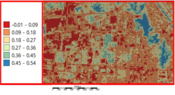
(8) 김윤기. Figure 3. Vectorized NDVI DATA Figure 2. the Spatial Distribution Pattern of NDVI Values. Local Geary Cluster Map, High-High, Low-Low, Other Positive, Negative, and Not Significant parts were selected in order and saved as separate shapefiles as well. Finally, in this study, shapefiles saved separately above were imported into QGIS and analyzed how the spatial distribution patterns of green spaces differed according to the analysis method. In this research, the QGIS ‘Intersection’ function was used to examine the difference between LISA and the Getis-Ord analysis results. Also, GRASS GIS’s ‘v.overlay’ feature was used to analyze the difference between LISA and the Local Geary C. QGIS’s ‘Intersection’ function was used to investigate the difference between the Getis-Ord’s analysis results and the Local Geary C’s analysis results.. 4. Results 4.1. NDVI and Vegetation Density Figure 2 shows the spatial distribution pattern of NDVI values. As can be seen from the figure, vegetation density was high in the eastern and. 32. 「지적과 국토정보」 제50권 제1호. 2020. central parts of the study area. Therefore, it can be seen that the green spaces are mainly distributed in the eastern and central regions of the research area. The spatial distribution pattern of green areas can be more easily identified using vectorized NDVI data rather than the image data. Figure 3 shows the vectorized NDVI data. Unlike Figure 2, Figure 3 divides the range of NDVI values into six sections at equal intervals of 0.09. By separating the NDVI values at equal intervals, researchers can more accurately identify the spatial distribution patterns of green spaces. Table 1 shows the distribution of pixels by the value interval. As can be seen from this table, the NDVI value in most of the study area is less than 0.18. It means that 62.01% of the study area is bare-soil or built-up areas. On the other hand, the region with the other hand, the region with an NDVI value of 0.18 or more occupies only 37.99% of the whole, so the vegetation density of the study area is not so high. In particular 1,278 pixels (12.2% of the total) had an NDVI value of 0.36 or more, indicating that there are not many good quality green areas or forests in this region..
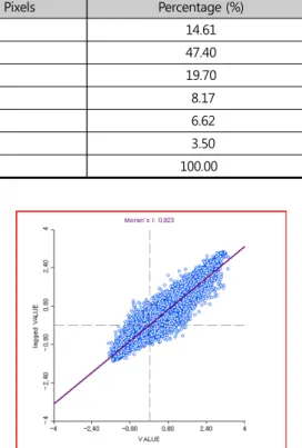
(9) A Study on the Spatial Distribution Patterns of Urban Green Spaces Using Local Spatial Autocorrelation Statistics. Table 1. the Distribution of Pixels by NDVI Value Interval NDVI Value Range. the Number of Pixels. Percentage (%). -0.01 – 0.09. 1,847. 14.61. 0.09 – 0.18. 5,991. 47.40. 0.18 – 0.27. 2,489. 19.70. 0.27 – 0.36. 1,033. 8.17. 0.36 – 0.45. 837. 6.62. 0.45 – 0.54. 441. 3.50. 12,638. 100.00. Total. 4.2. Spatial Distribution Patterns of Green Spaces 4.2.1. Local Moran’s I 1) Moran’s I Scatterplot The Moran Scatterplot shows the relationship between the selected attribute value at each position and the average value of the same attribute at adjacent locations (Anselin 1996). Figure 4. Figure 4. Moran’s I Scatterplot. shows the Moran scatterplot for the NDVI values. As can be seen from this figure, the Moran’s I. other hand, in the low-low cluster, the NDVI value. value for the data used in this study was very high. at each point and its local average value are both. at 0.823. It means that the NDVI values in the. lower than the overall average value of the NDVI.. study area form fairly distinct clusters. In this. And the spatial autocorrelation values of the. figure, the high-high cluster, or hotspot, is in the. high-high cluster and the low-low cluster are. first quadrant, and the low-low cluster, or colds-. both positive. On the other hand, the spatial. pot, is in the third quadrant. On the other hand,. autocorrelation values of the high-low cluster and. the high-low cluster is located in the second. the low-high cluster are both negative.. quadrant, and the low-high cluster is located in the fourth quadrant. Finally, the Not Significance. 2) LISA Cluster Map. cluster is found to be mostly concentrated in the. Figure 5 shows the LISA cluster map of NDVI.. center of the graph.. As can be seen in the figure, hotspots are located. In the high-high cluster, the NDVI value at each. mainly in the east, north, and central parts of the. point and its local average value are both higher. study area. The number of pixels in the hotspot. than the overall average value of the NDVI. On the. areas is 2,284, which is 18.07% of the total number Journal of Cadastre & Land InformatiX Vol.50 No.1 (2020). 33.
(10) 김윤기. Figure 5. LISA Cluster Map: NDVI. of pixels. These regions are dense vegetation forests or green spaces, with many positive effects on the surrounding industrial, business, and residential areas. In particular, the positive impact of forests and green spaces on the surrounding areas should be noted by policymakers and planners. However, coldspots were found to be distributed mainly in the west and south of the. Figure 6. LISA Significance Map of NDVI. these zones have a pleasant living environment because superior green regions surround apartment complexes and other development areas. If municipal governments or citizens manage well, these regions are likely to be promoted to hotspots in the future. However, the proportion of low-high clusters and high-low clusters in the study area was not found to be very high.. study area. Indeed, in these areas, the land is used as industrial areas, residential areas, and business areas, so the density of green spaces seems to be quite low. The number of pixels in the coldspot areas is 3,622, which is 28.66 of the total, which is considerably larger than the hotspot areas. However, clusters that city governments and city planners should pay attention to are low-high clusters and high-low clusters. First, high-low clusters are areas in which built-up areas surround green spaces with high vegetation density. These clusters are places where the development of the surrounding areas is highly likely to damage the. 3) LISA Significance Map Figure 6 shows the LISA Significance Map for NDVI values. In this study, 999 permutations and a p-value of 0.05 were used to produce the LISA significance map. As can be seen in Figure 6, there are 5,965 significant locations in the study area. Among these significant locations 2,369 sites were identified as statistically significant locations at a p-value of 0.001 1,642 pixels at a p-value of 0.01, and 1,955 positions at a p-value of 0.05, respectively. However, 6,673 sites were found to be statistically insignificant.. green zones. Therefore, these areas require considerable attention from policymakers and planners for the conservation and sustainable. 4.2.2. Local Getis-Ord . development of natural ecosystems. Low-high. 1) Cluster Map. clusters, on the other hand, face different. Figure 7 shows the cluster map for the. situations from high-low clusters. In other words,. spatial distribution of green spaces. Unlike the. 34. 「지적과 국토정보」 제50권 제1호. 2020.
(11) A Study on the Spatial Distribution Patterns of Urban Green Spaces Using Local Spatial Autocorrelation Statistics. Figure 7. Cluster Map. LISA cluster map, the cluster map divides urban green spaces into two clusters, high and low. Here, the high cluster of the cluster map corresponds to the high-high cluster of the LISA cluster map, but the number of locations belonging to this cluster is higher than that of the LISA cluster map. High clusters are located mainly in the east, north, and central areas of the research. Figure 8. Significance Map of NDVI. 4.2.3. Local Geary C Statistic 1) Local Geary Cluster Map Figure 9 shows the Local Geary cluster map of the spatial distribution of green spaces. As can be seen in this figure, high-high clusters (hotspots) are concentrated mainly in the east, north, and central regions of the study area. Also, 3,189 pixels. area. Also, low clusters in the cluster map. belonging to hotspots occupy a relatively high. correspond to low-low clusters in the LISA cluster. proportion of about 25.23% of the total research. map. The number of locations in this cluster was. area, which is quite different from other local. found to be bigger than the number of locations in. spatial autocorrelation techniques. Low-low clusters,. the low-low clusters of the LISA cluster map. Low. on the other hand, are evenly distributed throu-. clusters are concentrated in the west, south, and. ghout the study area, unlike other analytical. central regions of the study area. Also, as can be. methods. The number of pixels in coldspots was. seen in the figure, the 6,673 pixels were not. 5,465, which is much higher than other local. statistically significant.. autocorrelation techniques. In the Local Geary cluster map, other positive clusters and negative. 2) Significance Map. clusters are also identified. However, the number. Figure 8 shows the significance map for. of locations belonging to these two groups was. NDVI values. Nine hundred ninety-nine permuta-. minimal compared to hotspot clusters or coldspot. tions and a p-value of 0.05 were also used to. clusters.. produce the significance map. As can be seen from the figure, the significance map is the. 2) Local Geary Significance Map. same as the LISA significance map. These results. Figure 10 shows the Local Geary significance. suggest that the Local Moran’s statistic and the. map of the NDVI. In this study, 999 permutations. Local Getis-Ord statistic have almost similar results.. and a p-value of 0.05 were used to produce the Journal of Cadastre & Land InformatiX Vol.50 No.1 (2020). 35.
(12) 김윤기. Figure 9. Local Geary Cluster Map. Figure 10. Local Geary Significance Map. Local Geary significance map of the NDVI. As can. spatial distribution patterns of urban green spaces,. be seen in the figure, there are 9,300 significant. the p-value of all cluster maps was set to 0.05 and. locations in the study area. Among these pixels,. the permutations to 999, respectively. Furthermore,. 4,089 sites were identified as statistically signifi-. the performance of the LISA cluster map and the. cant locations at a p-value of 0.001 2,850 locations. cluster map were compared. The high-high. at a p-value of 0.01, and 2,355 positions at a. cluster of the LISA cluster map is similar to the. p-value of 0.05, respectively. These results are. high cluster of the cluster map, the low-low. quite different from the two analytical methods. cluster of the LISA cluster map corresponds to the. used in the above analysis to identify the spatial. low cluster of the cluster map, and the not. distribution patterns of green spaces. It is because. significant cluster of the LISA cluster map is. the Local Geary statistic uses a different approach. similar to the not significant cluster of the . to quantify attribute similarity than the Local. cluster map.. Moran or the Local statistics (Anselin 2019).. As a result of the overlay analysis (Table 2), the. That is, the weighted average of the neighbors. high-high cluster of the LISA cluster map and the. greatly influences the Local Moran and the Local. high cluster of the cluster map turned out to. statistics, but the squared difference affects the. have very high similarity. That is, the number of. Local Geary statistic, resulting in differences in. locations of the high-high cluster is 2,284, and the. analysis results between the local spatial auto-. number of pixels of the high group is 2,314, so the. correlation methods (Anselin 2019).. two clusters have no significant difference in the area. Each cluster has an intersection of 2,284. 4.3. Comparison of Local Spatial Autocorrelation Statistics. locations, indicating that both clusters are almost identical. Also, the similarity between the low-low cluster and low cluster was found to be very high.. 4.3.1. the LISA Cluster Map and the Cluster Map. That is, the number of pixels in the low-low cluster was 3,622, and the number of pixels in the. In this study, to find which spatial autocorre-. low cluster was 3,651, so the two groups have no. lation method performs better in identifying. significant difference in the size. Each of these. 36. 「지적과 국토정보」 제50권 제1호. 2020.
(13) A Study on the Spatial Distribution Patterns of Urban Green Spaces Using Local Spatial Autocorrelation Statistics. Table 2. The Number of Pixels Matched between LISA Clusters and the Clusters LISA Clusters. The Number of Pixels. Clusters. Number of Pixels. The Number of Pixels Matched. High-High. 2,284. High. 2,314. 2,284. Low-Low. 3,622. Low. 3,651. 3,622. Not Significant. 6,673. Not Significant. 6,673. 6,673. groups has an intersection of 3,622 pixels,. the Local Geary cluster map, and the not signifi-. signifying that both clusters are almost the same.. cant cluster of the Local Geary cluster map is. Moreover, the not significant cluster of LISA. equivalent to the not significant group in the Local. cluster map and the not significant cluster of the. Geary cluster map. As a result of the intersection. cluster map were 100 percent identical. That is,. analysis (Table 3), the high-high cluster of the. the number of pixels in the not significant clusters. LISA cluster map and the high-high group of the. of the two cluster maps was the same (6,673). The. Local Geary cluster map proved to have some. above comparison shows that there is a significant. differences. That is, the number of locations of the. similarity in terms of hotspots, cold spots, and the. high-high cluster for the LISA cluster map is. not significant clusters. However, not only hotspots. 2,284, and the number of pixels of the high-high. and coldspots but also spatial outliers play an. group for the Local Geary cluster map is 3,189, so. essential role in identifying spatial distribution. the two groups have some differences in the size.. patterns of green areas. In this respect, the LISA. Each group has an intersection of 2,061 locations,. cluster map, which has outlier clusters, is more. signifying that both groups are not the same.. effective than the cluster map in determining. Also, there were some differences between the. the spatial distribution pattern of the green spaces.. low-low cluster for the LISA cluster map and the low-low group for the Local Geary cluster map.. 4.3.2. The LISA cluster map and the Local Geary Cluster Map. That is, the number of pixels in the low-low cluster for the LISA cluster map was 3,622, and the. In this study, the performance of the LISA. number of locations in the low cluster for the. cluster map and the Local Geary cluster map in. Local Geary cluster map was 5,486, so the two. determining spatial distribution patterns of green. groups have some differences in the area. Each of. areas was compared and analyzed. And, the. these groups has an intersection of 3,310 pixels,. high-high cluster of the LISA cluster map is. indicating that both clusters are not identical.. similar to the high-high group of the Local Geary. The not significant cluster of the LISA cluster. cluster map, and the low-low cluster of the LISA. map and the not significant group of the Local. cluster map corresponds to the low-low cluster of. Geary cluster map turned out to have some. Journal of Cadastre & Land InformatiX Vol.50 No.1 (2020). 37.
(14) 김윤기. Table 3. The Number of Pixels Matched between the LISA Clusters and the Local Geary Clusters LISA Clusters. The Number of Pixels. Local Geary Clusters. Number of Pixels. The Number of Pixels Matched. High-High. 2,284. High-High. 3,189. 2,061. Low-Low. 3,622. Low-Low. 5,486. 3,310. Not Significant. 6,673. Not Significant. 3,338. 2,758. Table 4. The Number of Pixels Matched between the Clusters and the Local Geary Clusters. Clusters. Local Geary Clusters. High. 2,314. High-High. 3,189. 2,061. Low. 3,651. Low-Low. 5,486. 3,310. Not Significant. 6,673. Not Significant. 3,338. 2,758. differences. That is, the number of pixels of the. Number of Pixels. The Number of Pixels Matched. The Number of Pixels. outliers.. not significant cluster for the LISA cluster map is 6,673, and the number of pixels of the not significant group for the Local Geary cluster map. 4.3.3. The Cluster Map and the Local Geary Cluster Map. is 3,383, so the two clusters have some differences. In this study, the performance of the cluster. in the area. Each cluster has an intersection of. map and the Local Geary cluster map in identi-. 3,310 locations, signifying that both groups are not. fying the spatial distribution pattern of the green. the same in terms of the not significant clusters.. spaces was compared (Table 4). The high cluster. As discussed above, there were some differences. of the cluster map is similar to the high-high. between the clusters of the LISA cluster map and the clusters of the Local Geary cluster map. The reason is that the Local Moran and Local GI statistics are greatly influenced by the weighted average of neighbors, while the Local Geary method is affected by the squared difference (Anselin 2019). Also, to properly analyze the spatial distribution patterns of green areas and propose policy alternatives, city planners and policymakers must identify not only hotspots and coldspots but also spatial outliers. From this point of view, the LISA cluster map outperforms the Local Geary cluster map in identifying spatial. 38. 「지적과 국토정보」 제50권 제1호. 2020. cluster of the Local Geary cluster map, the low cluster of the cluster map corresponds to the low-low cluster of the Local Geary cluster map, and the not significant cluster of the cluster map is similar to the not significant cluster of the Local Geary cluster map. As a result of the overlay analysis, the high cluster of the cluster map and the high-high group of the Local Geary cluster map turned out to have some differences. That is, the number of pixels of the high cluster for the cluster map is 2,314, and the number of locations of the high-high group for the Local.
(15) A Study on the Spatial Distribution Patterns of Urban Green Spaces Using Local Spatial Autocorrelation Statistics. Geary cluster map is 3,189, so the two groups have. makers have to precisely identify the spatial. some differences in the size. Each cluster has an. distribution patterns of the green spaces and. intersection of 2,061 locations, indicating that both. propose appropriate solutions for each cluster to. groups are not the same.. solve problems related to the green spaces. First,. Also, there were some differences between the. for high-high groups, policymakers will have to. low cluster for the cluster map and the low-. focus on preservation and management to ensure. low group for the Local Geary cluster map. That is,. that the green spaces and forests are not damaged. the number of locations in the low cluster for the. in the future. The green spaces located in the. cluster map was 3,651, and the number of. hotspots of the research area not only provide. locations in the low cluster for the Local Geary. citizens with places to relax but also act as cooling. cluster map was 5,486, so the two groups have. islands that cool down the warm air caused by. some differences in the area. Each of these groups. global warming. Therefore, planners and policymakers. has an intersection of 3,310 pixels, indicating that. must focus their attention on fostering and. both groups are not the same. The not significant. preserving healthy green spaces. The management. cluster of the cluster map and the not signifi-. of coldspot clusters is just as important as the. cant group of the Local Geary cluster map proved. management of hotspot clusters. Low-low groups. to have some differences. That is, the number of. act as heat islands that increase the surface. locations of the not significant cluster for the . temperature in summer, which has a significant. cluster map is 6,673, and the number of pixels of the not significant group for the Local Geary cluster map is 3,383, so the two clusters have some differences in the size. Each cluster has 2,758 overlaps of locations, indicating that both groups are not the same in terms of the not significant clusters. The above overlay analysis shows that there are some differences in terms of hotspots, cold spots, and the not significant clusters.. impact on the climate ecosystem of the surrounding areas. To overcome these coldspot problems, policymakers and planners should focus their attention on the greening of these areas. In particular, the roof greening projects not only lower the temperature of the low-low clusters but also provide clean air to the residents living in the surrounding areas. However, policymakers should focus more attention on low-high clusters and high-low clusters. In particular, high-low clusters are areas. 5. Discussion. with high potential for damage to the green spaces and forests in the future. In other words, since. The study area is located in the west of Cheongju. these areas are clusters where development areas. city, where industrial, business, and residential. are located around the green spaces or woods, it is. functions are mixed, and the green spaces have. necessary to regulate development activities. been severely damaged. Urban planners and policy-. around green fields and forests strictly. The city Journal of Cadastre & Land InformatiX Vol.50 No.1 (2020). 39.
(16) 김윤기. we live in today is a place of life not only for our. respect, the LISA cluster map, which has outlier. generation but also for our descendants. Therefore,. clusters, is more effective than the cluster map. policymakers and city planners should carry out. and the Local Geary cluster map in determining. urban development. carefully. the spatial distribution pattern of the green. reviewing their impact on the surrounding. spaces. Therefore, to properly analyze the spatial. environment. However, low-high clusters are. distribution patterns of green areas and propose. clusters that face the opposite situation of. policy alternatives, city planners and policymakers. high-low clusters. These areas are excellent. must identify not only hotspots and coldspots but. places to live because the remarkable green spaces. also spatial outliers.. projects. after. surround the apartment complexes or detached. This study can contribute to the research on the. housing complexes. These clusters will play a key. spatial distribution patterns of the green spaces in. role in conserving green spaces in the future.. the following aspects. First, this research differs. Policymakers and urban planners will, therefore,. from previous studies in that it uses not only. have to do their best to preserve and sustainably. image analysis but also local spatial autocorrela-. develop the areas.. tion techniques in identifying spatial distribution patterns of the green spaces. In particular, this. 6. Conclusion. study can contribute to the related-fields in that it vectorized the NDVI images, and then it analyzed. The primary purpose of this study was to compare. the spatial distribution patterns of the green. and analyze the performance of local spatial. spaces using local spatial autocorrelation techniques.. autocorrelation techniques in identifying spatial. Second, this research may contribute to the. distribution patterns of the green areas. First, the. related-fields in that it compared the performance. LISA cluster map and the cluster map showed. of the Local Geary cluster map, the cluster map,. high similarity in discovering hotspots, coldspots,. and the Local Geary cluster map in determining. and not significant clusters. However, the LISA. spatial distribution patterns of the green spaces.. cluster map and the Local Geary cluster map did. Despite these differences and usefulness, this. not reveal considerable similarity in determining. study has the following limitations. Since this. different clusters of the green spaces. The . study used Landsat 8 image with a spatial. cluster map and the Local Geary cluster map also. resolution of 30m as the primary data, it could not. didn't display significant similarity in identifying. identify a more detailed spatial distribution. different groups of green areas. However, not only. pattern of the green areas. In future work, this. hotspots and coldspots but also spatial outliers. limitation can be overcome by using Sentinels or. play an essential role in identifying spatial. UAV images with high spatial resolution. Second,. distribution patterns of the green zones. In this. this study used only NDVI to identify spatial. 40. 「지적과 국토정보」 제50권 제1호. 2020.
(17) A Study on the Spatial Distribution Patterns of Urban Green Spaces Using Local Spatial Autocorrelation Statistics. distribution patterns of the green spaces. Therefore,. Bao T, Li X, Zhang J, Zhang Y, Tian S. 2016.. the explanatory power of those models used in this. Assessing the distribution of urban green. research may be lower than when several vegeta-. spaces and its anisotropic cooling distance on. tion indices are used simultaneously. In future. urban heat island pattern in Baotou. China.. research, it may be a good research topic to. ISPRS International Journal of Geo-Infor-. analyze the spatial distribution patterns of green. mation. 5(2):12.. areas using various vegetation indices, and then examine how the results differ.. Baruch-Mordo, Breck SW, Wilson KR, Theobald DM. 2008. Spatiotemporal distribution of black bear‐human conflicts in Colorado. USA. The. References Abelt K, McLafferty S. 2017. Green streets: urban green and birth outcomes. International journal. of environmental research and public health. 14(7):771. Anguluri R, Narayanan P. 2017. Role of green space in urban planning: Outlook towards smart cities. Urban Forestry & Urban. Greening. 25:58-65. Anselin L. 1995. Local indicators of spatial association-LISA. Geographical analysis. 27(2): 93-115. Anselin L, 2019. A local indicator of multivariate spatial association: extending Geary’s C.. Geographical Analysis. 51(2):133-150. Anselin L, Syabri I, Kho Y. 2006. GeoDa: an introduction to spatial data analysis. Geogra-. phical analysis. 38(1):5-22. Avdan U, Jovanovska G. 2016. Algorithm for automated mapping of land surface temperature using LANDSAT 8 satellite data.. Journal of Sensors. Bao S, Henry M. 1996. Heterogeneity issues in local measurements of spatial association. Geogra-. phical Systems. 3:1-14.. Journal of Wildlife Management. 72(8):18531862. Bhatti SS, Tripathi NK. 2014. Built-up area extraction using Landsat 8 OLI imagery.. GIScience sensing. 51(4):445-467. Bivand R. 2002. Spatial econometrics functions in R: Classes and methods. Journal of geogra-. phical systems. 4(4):405-421. Bivand R. 2006. Implementing spatial data analysis software tools in R. Geographical Analysis. 38(1):23-40. Bivand R. 2009. Applying measures of spatial autocorrelation: computation and simulation.. Geographical Analysis. 41(4):375-384. Carlson TN, Ripley DA. 1997. On the relation between NDVI. fractional vegetation cover. and leaf area index. Remote sensing of En-. vironment. 62(3):241-252. Cima EG, Uribe-Opazo MA, Johann JA, Rocha Jr WFD, Dalposso GH. 2018. Analysis of spatial autocorrelation of grain production and agricultural storage in Parana. Engenharia. Agrícola. 38(3):395-402. Dalposso GH, Uribe-Opazo MA, Mercante E, Lamparelli RA. 2013. Spatial autocorrelation of NDVI and GVI indices derived from Landsat/ Journal of Cadastre & Land InformatiX Vol.50 No.1 (2020). 41.
(18) 김윤기. TM images for soybean crops in the western. Getis A. 2008. A history of the concept of spatial. of the state of Paraná in 2004/2005 crop. autocorrelation: A geographer’s perspective.. season. Engenharia Agrícola. 33(3):525-537.. Geographical Analysis. 40(3):297-309.. de México CE. 2017. Spatial modeling of forest. Haaland C, van den Bosch CK. 2015. Challenges. fires in Mexico: an integration of two sources.. and strategies for urban green-space planning. Bosque. 38(3):563-574.. in cities undergoing densification: A review.. Dwyer MC, Miller RW. 1999. Using GIS to assess urban tree canopy benefits and surrounding greenspace distributions. Journal of Arboricul-. ture. 25:102-107.. Urban forestry & urban greening. 14(4): 760-771. Han TTN, Hoa PK, Khoa HB, Van TT. 2018. Understanding Satellite Image-Based Green. El-Gammal MIARR, Samra RA. 2014. NDVI. Space Distribution for Setting up Solutions on. threshold classification for detecting vegetation. Effective Urban Environment Management. In. cover in Damietta governorate. Egypt. Journal. Multidisciplinary Digital Publishing Institute. of American Science. 10(8):108-113.. Proceedings. 2(10):570.. Fu WJ, Jiang PK, Zhou GM, Zhao KL. 2014. Using. Hoffimann E, Barros H, Ribeiro A. 2017. Socio-. Moran’s I and GIS to study the spatial pattern. economic inequalities in green space quality. of forest litter carbon density in a subtropical. and accessibility—Evidence from a Southern. region of southeastern China. Biogeosciences.. European city. International journal of en-. 11(8):2401-2409.. vironmental research and public health.. Gamon JA, Field CB, Goulden ML, Griffin KL,. 14(8):916.. Hartley AE, Joel G, Valentini R. 1995. Rela-. Jacquez GM. 2000. Spatial analysis in epide-. tionships between NDVI. canopy structure.. miology: Nascent science or a failure of. and photosynthesis in three Californian. GIS?. Journal of Geographical Systems. 2(1):. vegetation types. Ecological Applications. 5(1):. 91-97.. 28-41.. Jennings V, Larson L, Yun J. 2016. Advancing. Gandhi GM, Parthiban S, Thummalu N, Christy A.. sustainability through urban green space:. 2015. NDVI: vegetation change detection. Cultural ecosystem services. equity. and social. using remote sensing and GIS–a case study of. determinants of health. International Journal. Vellore District. Procedia Computer Science.. of environmental research and public health.. 57:1199-1210.. 13(2) 196.. Georgi JN, Dimitriou D. 2010. The contribution of. Keller W, Shiue CH. 2007. The origin of spatial. urban green spaces to the improvement of. interaction. Journal of Econometrics. 140(1):. environment in cities: Case study of Chania.. 304-332.. Greece. Building and environment. 45(6):14011414.. 42. 「지적과 국토정보」 제50권 제1호. 2020. Kong F, Yin H, Nakagoshi N, Zong Y. 2010. Urban green space network development for bio-.
(19) A Study on the Spatial Distribution Patterns of Urban Green Spaces Using Local Spatial Autocorrelation Statistics. diversity conservation: Identification based. adaptation. ISPRS Journal of Photogrammetry. on graph theory and gravity modeling. Land-. and Remote Sensing. 89:59-66.. scape and urban planning. 95(1-2):16-27.. Majumdar DD, Biswas A. 2016. Quantifying land. Kosfeld R, Lauridsen J. 2012. Identifying clusters. surface temperature change from LISA clusters:. within R&D intensive industries using local. An alternative approach to identifying urban. spatial methods.. land use transformation. Landscape and Urban. Lee SI. 2001. Developing a bivariate spatial asso-. Planning. 153:51-65.. ciation measure: an integration of Pearson’s r. McCauley LA, Jenkins DG. 2005. GIS‐based. and Moran’s I. Journal of geographical. estimates of former and current depressional. systems. 3(4):369-385.. wetlands in an agricultural landscape. Ecolo-. Le Gallo J, Ertur C. 2003. Exploratory spatial data. gical Applications. 15(4):1199-1208.. analysis of the distribution of regional per. McConnachie MM, Shackleton CM. 2010. Public. capita GDP in Europe 1980–1995. Papers in. green space inequality in small towns in South. regional science. 82(2):175-201.. Africa. Habitat International. 34(2):244-248.. Leung Y, Mei CL, Zhang WX. 2003. Statistical test. M’Ikiugu MM, Kinoshita I, Tashiro Y. 2012. Urban. for local patterns of spatial association.. green space analysis and identification of its. Environment and Planning A. 35(4):725-744.. potential expansion areas. Procedia-Social. Levine N. 2013. Hot spot analysis of zones. N. and Behavioral Sciences. 35:449-458.. Levine. CrimeStat: Spatial Statistics Program. Myint SW, Wentz EA, Purkis SJ. 2007. Employing. for the Analysis of Crime Incident Locations.. spatial metrics in urban land-use/land-cover. Version. 4 242960-242995.. mapping. Photogrammetric Engineering &. Lwin K, Murayama Y. 2009. A GIS Approach to. Remote Sensing. 73(12):1403-1415.. Estimation of Building Population for Micro‐. Noce S, Collalti A, Valentini R, Santini M. 2016. Hot. spatial Analysis. Transactions in GIS. 13(4):. spot maps of forest presence in the Mediter-. 401-414.. ranean basin. iForest-Biogeosciences and. Machiwal D, Mishra A, Jha MK, Sharma A, Sisodia. Forestry. 9(5):766.. SS. 2012. Modeling short-term spatial and. Ord JK, Getis A. 1995. Local spatial autocorrelation. temporal variability of groundwater level. statistics: distributional issues and an appli-. using geostatistics and GIS. Natural resources. cation. Geographical analysis. 27(4):286-306.. research. 21(1):117-136.. Orner I, Benenson I. 2002. Investigating fine-scale. Maimaitiyiming M, Ghulam A, Tiyip T, Pla F,. residential segregation by means of local. Latorre-Carmona P, Halik Ü, Caetano M. 2014.. spatial statistics. In Geography Research Forum.. Effects of green space spatial pattern on land. 22:41-60.. surface temperature: Implications for sustainable urban planning and climate change. Peng L. 1987. DISTRIBUTION OF MANGROVE SPECIES [J]. Scientia Silvae Sinicae. 4. Journal of Cadastre & Land InformatiX Vol.50 No.1 (2020). 43.
(20) 김윤기. Pernas JB. García MLL. 2015. Modelling spatial patterns and temporal trends of wildfires in Galicia (NW Spain). Forest Systems. 24(2):1. Pettorelli N, Vik JO, Mysterud A, Gaillard JM,. Health. 9(1):464. Tucker CJ, Pinzon JE, Brown ME, Slayback DA, Pak EW, Mahoney R, El Saleous N. (2005). An extended. AVHRR 8‐km NDVI. dataset. Tucker CJ, Stenseth NC. 2005. Using the. compatible with MODIS and SPOT vegetation. satellite-derived NDVI to assess ecological. NDVI data. International Journal of Remote. responses to environmental change. Trends. Sensing. 26(20):4485-4498.. in ecology & evolution. 20(9):503-510.. Waldhör T. 1996. The spatial autocorrelation. Rouse Jr J, Haas RH, Schell JA, Deering DW. 1974.. coefficient Moran’s I under Heterosceda-. Monitoring vegetation systems in the Great. sticity. Statistics in Medicine. 15(7-9): 887-. Plains with ERTS.. 892.. Shackleton S, Chinyimba A, Hebinck P, Shackleton. Wang J, Xu C, Pauleit S, Kindler A, Banzhaf E.. C, Kaoma H. 2015. Multiple benefits and. 2019a. Spatial patterns of urban green infra-. values of trees in urban landscapes in two. structure for equity: A novel exploration.. towns in northern South Africa. Landscape. Journal of Cleaner Production. 238:117858.. and Urban Planning. 136:76-86.. Wang WC, Chang YJ, Wang HC. 2019b. An. Sokal RR, Oden NL, Thomson BA. 1998. Local. Application of the Spatial Autocorrelation. spatial autocorrelation in a biological model.. Method on the Change of Real Estate Prices in. Geographical Analysis. 30(4):331-354.. Taitung City. ISPRS International Journal of. Tian Y, Jim CY, Tao Y, Shi T. 2011. Landscape. Geo-Information. 8(6):249.. ecological assessment of green space frag-. Wen M, Zhang X, Harris CD, Holt JB, Croft JB. 2013.. mentation in Hong Kong. Urban Forestry &. Spatial disparities in the distribution of parks. Urban Greening. 10(2):79-86.. and green spaces in the USA. Annals of. Tiefelsdorf M. 2002. The saddlepoint approxi-. Behavioral Medicine. 45(suppl_1):S18-S27.. mation of Moran’s I’s and local Moran’s Ii’s. Wüstemann H, Kalisch D, Kolbe J. 2017. Access to. reference distributions and their numerical. urban green space and environmental ine-. evaluation. Geographical Analysis. 34(3):187-. qualities in Germany. Landscape and Urban. 206.. Planning. 164:124-131.. Truong LT. Somenahalli SV. 2011. Using GIS to. Xu D, Guo X. 2014. Compare NDVI extracted from. identify pedestrian-vehicle crash hot spots. Landsat 8 imagery with that from Landsat 7. and unsafe bus stops. Journal of Public. imagery. American Journal of Remote Sensing.. Transportation. 14(1):6.. 2(2):10-14.. Tsai PJ, Lin ML, Chu CM, Perng CH. 2009. Spatial care. based traffic analysis zone design: implemen-. hotspots in Taiwan in 2006. BMC Public. tation and evaluation. Transportation Planning. autocorrelation. 44. You J. Nedović‐Budić Z. Kim TJ. 1998. A GIS‐. analysis. of. health. 「지적과 국토정보」 제50권 제1호. 2020.
(21) A Study on the Spatial Distribution Patterns of Urban Green Spaces Using Local Spatial Autocorrelation Statistics. and Technology. 21(1-2):69-91.. urban green space: A conceptual framework of valuation and accessibility measurements.. Zhang H, Xue L, Yang C, Chen X, Zhang L, Wei G.. Management of Environmental Quality.. 2018. Dynamic Assessment on the Landscape Patterns and Spatio-temporal Change in the mainstream of Tarim River. In IOP Con-. ference Series: Earth and Environmental. 2020년 02월 21일 원고접수(Received). Science. 108(3):032058. IOP Publishing.. 2020년 05월 08일 1차심사(1st Reviewed). Zhou X, Parves Rana M. 2012. Social benefits of. 2020년 06월 12일 게재확정(Accepted). 초 록 본 연구의 주된 목적은 녹지의 공간 분포 패턴을 식별하는데 있어 국지적 공간자기상관 기법들의 성능을 비교하고 분석하는 것이다. 이 연구목적을 달성하기 위해 본 연구는 위성영상분석기법과 공간 자기상관기법들을 이용하였다. 분석의 결과 공간 특이치 군집을 갖는 LISA 군집지도가 도시녹지의 공 간 분포 패턴을 식별하는 데 있어서 다른 분석기법들보다 우수함이 확인되었다. 본 연구는 기존의 연 구들과는 다른 몇 가지 연구방법을 이용했다는 점에서 관련분야에 기여할 수 있다. 이러한 차별성과 유용성에도 불구하고 본 연구는 녹지의 공간적 분포패턴을 식별하는 있어서 저해상도 위성영상을 이 용했다는 점과 식생지수들 중에서 NDVI만을 이용했다는 점에서 한계를 지닌다. 이러한 한계들은 향 후연구에서 UAV영상을 이용하거나 또는 여러 가지 식생지수들을 동시에 이용한다면 극복될 수 있을 것이다. 주요어 : 녹지, 공간적, 분포, 패턴, 공간자기상관, LISA, NDVI. Journal of Cadastre & Land InformatiX Vol.50 No.1 (2020). 45.
(22)
수치


+3
관련 문서
Abstract: This study was conducted to develop a carbon storage distribution map of Pinus rigida stands in Muju-gun by using of the National Forest Inventory data and digital
This study is to analyze spatial distribution and characteristics of phenology changes using MODIS images.. It can figure out changes of phenology by
This study compares and analyzes the spatial distribution of people in two cities using location information in twitter data.. The target cities were selected as Paris, a
This study developed a method for calculating relevant length of left turn storage lengths based on an empirical arriving distribution at signalized intersections in
A Study on the Urban Spatial Structure Change in Population Growth Type Local Medium Sized City: A Case of Asan-si* Hyongsang Lee* 요약 : 본 연구는 인구가
Also, by using IDW method among spatial interpolation methods of GIS, monthly and time-slot distribution maps were constructed, and based on this, spatial
Next, GWR(Geographically Weighted Regression) was used to analyze the spatial relations between the distribution of small business, hourly mobile
The purpose of this study is to evaluate preferences for spatial composition by urban design guidelines of detached housing areas using CG simulation, with the aim of
