https://doi.org/10.7848/ksgpc.2018.36.3.153
A Study on Calculating Relevant Length of Left Turn Storages Using UAV Spatial Images Considering Arrival Distribution
Characteristics at Signalized Intersections in Urban Commercial Areas
Yang, Jaeho
1)ㆍKim, Eungcheol
2)ㆍNa, Young-Woo
3)ㆍChoi, Byoung-Gil
4)Abstract
Calculating the relevant length of left turn storages in urban intersections is very crucial in road designs.
A left turn lane consists of deceleration lanes and left turn storages. In this study, we developed methods for calculating relevant lengths of left turn storages that vary at each intersection using UAV (Unmanned Aerial Vehicle) spatial images. Problems of conventional design techniques are applying the same number of left turn vehicles (N) using Poisson distribution without considering land use types, using a vehicle length that may not be measurable when applying the length of waiting vehicles (S), and using same storage length coefficient (α), 1.5, for every intersections. In order to solve these problems, we estimated the number of left turn vehicles (N) using an empirical distribution, suggested to use headways of vehicles for (S) to calculate the length of waiting vehicles (S) with a help of using UAV spatial images, and defined ranges of storage length coefficient (α) from 1.0 to 1.5 for flexible design. For more convenient design, it is suitable to classify two cases when possible to know and impossible to know about ratio of large trucks among vehicles when planning an intersection. We developed formula for each case to calculate left turn storage lengths of a minimum and a maximum. By applying developed methods and values, more efficient signalized intersection operation can be accomplished.
Keywords : Urban Commercial Intersections, Left Turn Storages, UAV Spatial Images, Empirical Distributions, Headways, Storage Length Coefficients
Original article
Received 2018. 05. 15, Revised 2018. 06. 14, Accepted 2018. 06. 26
1) Dept. of Civil and Environmental Engineering, Incheon National University (E-mail: [email protected])
2) Corresponding Author, Member, Dept. of Civil and Environmental Engineering, Incheon National University (E-mail: [email protected]) 3) Member, Dept, Hub-industrial-Academic Cooperation, Incheon National University (E-mail: [email protected])
4) Member, Dept. of Civil and Environmental Engineering, Incheon National University (E-mail: [email protected])
This is an Open Access article distributed under the terms of the Creative Commons Attribution Non-Commercial License (http://
1. Introduction
1.1 Purposes and backgrounds of this study
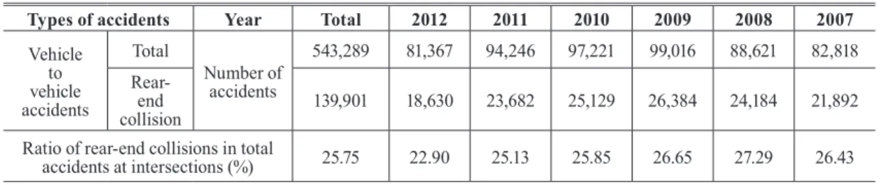
There are many reasons causing the rear-end collisions at urban signalized intersections. Among them, one of the critical reasons is the spill-back phenomenon of left turn vehicles due to shortages of left turn storage lengths.Actually, TAAS (Traffic Accident Analysis System) in South Korea showed that the rear-end collision is over 25 % in
signalized intersection accidents during 6 years from 2007 to 2012 as shown in Table 1 (KoROAD, 2015).
This means that rear-end accidents can be reduced if a relevant left turn storage length is offered. Providing a relevant left turn storage length in urban commercial areas is very crucial since it is connected with efficient usage of urban spaces and a budget. But, the methods for calculating a relevant left turn storage length are not developed concretely.
This study tries to develop the methods for calculating a
A left turn lane (L) consist of a left turn storage length (Ls) and a deceleration length (Ld) as shown in Eq. (1).
L = Ls + Ld (1)
Ls can be obtained by multiplying a storage length coefficient (α), the number of arriving vehicles (N), and the length of waiting vehicles (S) as shown in Eq. (2).
Ls = α × N × S (2)
As to α, the values of 1.5 and 2.0 are used for signalized and unsignalized intersections, respectively. N is the number of arriving vehicles within 1 cycle for signalized intersections, or within 1 minute for unsignalized intersection.
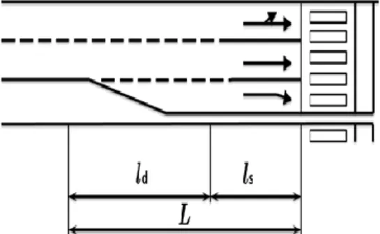
In the case of Japan, a similar method applies. Calculating formula of right turn lane length in Japan is shown in Eq. (3) (JRA, 2005).
L = ℓd + ℓs (3)
L is the length of right turn lane, ℓd is the length of taper, Fig. 1. Details of design rules of left turn storages relevant left turn storage length and to suggest a design
manual that can be adaptable at signalized intersections in urban commercial areas using UAV (Unmanned Aerial Vehicle) spatial images.
The South Korea design manual suggests calculating a left turn storage length by multiplying three variables such as a storage length coefficient, the number of left turn vehicles, and the length of waiting vehicles. This method, however, is not clear enough in terms of how to count the number of left turn vehicles, how to measure the length of waiting vehicles, and what storage length coefficients to apply at real situations.
1.2 Scope and research flow
Urban intersections have variable shapes. Target intersections of the study are 4-leg urban intersections having only one left turn lane and 4 or 6 through lanes located in commercial areas. AM peak hour is selected for surveying time. Among 60 intersections in database systems of urban traffic volume survey in South Korea (Incheon metropolitan city, 2009), three intersections (Seokbawi, Su- in, Sungeuisijang) are selected as study intersections after checking out the land use maps.
Research flow contains introduction, literature review, problem identifications, developing a new method, and applying the new methodology followed by conclusions.
2. Literature Review
2.1 Left turn lanes on design manual of each country
Fig. 1 shows elements of left turn design on South Korea road design manual (KSCE, 2009).
Table 1. Comparing ratio of rear-end collisions in total accidents at intersections
Types of accidents Year Total 2012 2011 2010 2009 2008 2007
Vehicle vehicle to accidents
Total
Number of accidents
543,289 81,367 94,246 97,221 99,016 88,621 82,818 Rear-
collisionend 139,901 18,630 23,682 25,129 26,384 24,184 21,892
Ratio of rear-end collisions in total
accidents at intersections (%) 25.75 22.90 25.13 25.85 26.65 27.29 26.43
and ℓs is the length of storage lane as shown in Fig. 2.
ℓs can be obtained by multiplying a storage length coefficient (λr), the number of arriving vehicles (N) per 1 cycle, and the average headway (S) as shown in Eq. (4).
ℓs = λr × N × S (4)
A Policy on Geometric Design of Highways and Streets (AASHTO, 2011) says that a left turn lane consists of decelerating length of left turn lane, a taper, and a storage lane. At unsignalized intersections, the storage length should be determined by average arriving vehicles within 2 minutes at peak hours, or at least the length of 2 vehicles when the ratio of heavy vehicles is more than 10 %. At signalized intersections, the storage length should be based on one or one and half times to arriving vehicles. Even more, the storage length can be expanded to two times to arriving vehicles.
Urban Street Geometric Design Handbook (ITE, 2008) suggests to look up Urban Intersection Design Guide (TxDOT, 2005) about left turn lane designs. Urban Intersection Design Guide explains that left turn lane length is consist of decelerating length of left turn lane, a taper, and a storage lane, similar explanation to A Policy on Geometric Design of Highways and Streets (AASHTO, 2011).
2.2 Left turn lanes and U-Turns on papers and guidelines
Qi et al. (2007) developed a method for estimating the
storage lengths of left-turn lanes at signalized intersections.
The method was based on the discrete-time Markov chain simulation considering arrival rates and service rates of intersections. Kim (2002) calculated the length of storage and headways according to U-Turn existence. Lee (2009) pointed out problems about using Poisson distribution. He counted the number of observed vehicles after classifying intersections according to U-turn existence, and found that negative binomial distribution is more appropriate to explain arriving characteristics. When applying negative binomial distribution instead Poisson distribution, it is also found that the length of storage lane is calculated longer.
MNDOT (2008) developed formulas for calculating the storage lane length by classifying left turns into protected, permitted and yield as shown in Table 2.
Fig. 2. Right turn lane length suggested in guidelines for road structures in Japan
Speed Storage length
Deceler-
ation Taper Storage length
30 170 100 LTprot
= 35.3 + 0.0203*TV + 1.14*LTV - 0.171*Sp - 6.75*HVT + 1.32*HVL - 0.16*Gr LTperm
= 45.2 - 0.00953*TV + 0.0406*OV + .610*LTV + 0.348*Sp + 0.812*HVT+
1.76*HVL + 0.35*Gr LTyield
= 0.00 + 0.00315*TV + 0.0332*OV + 0.345*LTV - 0.149*Sp + 0.224*HVT + 0.629*HVL - 0.080*Gr
35 170 100
40 275 130
45 340 130
50 410 130
55 485 130
60 485 130
65 485 130
70 485 130
TV : Through Vehicles LTV : Left Turn Vehicles Sp : Speed
Gr : Grade
HVT : Heavy Vehicle Through HVL : Heavy Vehicle Left Turn OV : Opposite vehicle
Table 2. Models for left turn lane lengths by MNDOT
3. Problem Identification and Finding Improved Methodology
As mentioned above, Problems of existing design techniq- ues are applying the same number of left turn vehicles (N) using Poisson distribution without considering land use types, using a vehicle length that may not be measurable when applying the length of waiting vehicles (S), and using same storage length coefficient (α), 1.5 for every signalized intersections.
3.1 Finding improved methodology
To get the number of arriving vehicles at signalized intersections, most cases apply Poisson distribution as shown in Eq. (5).
(5)
where, x is the number of arrival vehicles in a given unit time, P(x) is arrival probability that x vehicles occur, and m is the average number of left turn vehicles in one unit time. Mean and variance of x are m. As all know, Poisson distribution is only suitable for the events that are random and rare (Do, 2005). Therefore, using Poisson distribution is not relevant to apply urban intersections specially in commercial areas. Indeed, it is very hard to find a suitable distribution model to fit into real situations.
This study suggests using an empirical distribution. In many situations we might want to use the observed data themselves to specify directly (in some sense) a distribution, called an empirical distribution, from which random values are generated during the simulation, rather than fitting a theoretical distribution to the data (Law and Kelton, 2007).
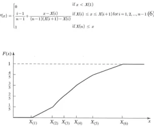
For continuous random variables, the type of empirical distribution that can be defined depends on whether we have the actual values of the individual original observations X1, X2, ..., Xn rather than only number of X(i)'s that fall into each of several specified intervals. Let X(i) denote the ith smallest of the Xj's, so that X(1) ≤ X(2) ≤ ... ≤ X(n). Then F is given by Eq. (6). Fig. 3 gives an illustration for n=6.
(6)
3.2 Methodology for improvement getting the length of waiting vehicle (S)
In Eq. (2), the length of waiting vehicles can be only obtained by observation. Then, the design value of lengths, S, might be an average value or a sum of every observed vehicle type lengths.
In existing methods, 7 m is used for an average value and 6 m for passenger cars and 12.0 m for trucks. This procedure does not consider the spacing between vehicles causing shorter length of storage lanes.
Therefore, this study suggests to apply the average headway based on empirical distribution of arriving vehicles and using UAV spatial images instead of using the length of vehicles.
3.3 Methodology for selecting the values of storage length coefficients
As mentioned earlier, the values of storage length coefficients (α) are 1.5 for signalized intersections and 2.0 for unsignalized intersections. This method is too strict and not efficient to various intersections in urban commercial areas.
This study suggests to use different values for each intersection considering different environments discussed later.
Fig. 3. Empirical cumulative distribution illustration when n=6
4. Application of Developed Methodology 4.1 The number of left turn vehicles (N) at
signalized intersections
To get the number of left turn vehicles by building up empirical distribution, field survey should be preceded.
We had field surveyed intersections satisfying 4-leg, no U-turns, only one left turn lane, and four or six through traffic lanes located in commercial areas. Within 60 intersections, we found only three signalized intersections
satisfying conditions mentioned, Seokbawi, Su-in, and Sungeuisijang intersections located in Incheon metropolitan city, South Korea. Characteristics of field investigation for study intersections are shown in Table 3.
Based on field survey, we collected data such as the number of arrival vehicles per cycle, observation frequency per cycle, total volume, observation probability, accumulated observation frequency and accumulated observation probability as shown in Table 4.
Classification Investigation date
and time Investigation direction Signal
cycle Left turn time Seokbawi
intersection 7/4/2013 (Fri)
07:30~08:30 Gyeonginno (old civic center intersection) →
Gyeonginno (direction to Seokam intersection) 170 sec 30 sec Su-in intersection 7/8/2013 (Mon)
07:15~08:15 Injoongno (Shinkwang intersection) →
Seohaedaero (direction to Lotte mart) 160 sec 30 sec Sungeuisijang
intersection 9/27/2013 (Tue)
08:00~09:00 Chamwoijunno (Enterance of Namgu office three legs
intersection) → Sukjungro (Soongeui rotary) 160 sec 30 sec Table 3. Characteristics of study intersections through field investigation
Classification Number of
vehicle/cycle Observation
frequency Total volume Observation probability
Accumulated observation
frequency
Accumulated observation
probability
Seokbawi intersection
0 0 0 0 0 0
1 0 0 0 0 0
2 0 0 0 0 0
3 0 0 0 0 0
4 0 0 0 0 0
5 0 0 0 0 0
6 0 0 0 0 0
7 0 0 0 0 0
8 2 16 0.095238 2 0.095238
9 0 0 0 2 0.095238
10 0 0 0 2 0.095238
11 3 33 0.142857 5 0.238095
12 2 24 0.095238 7 0.333333
13 1 13 0.047619 8 0.380952
14 2 28 0.095238 10 0.47619
15 4 60 0.190476 14 0.666667
16 2 32 0.095238 16 0.761905
17 2 34 0.095238 18 0.857143
18 2 36 0.095238 20 0.952381
19 0 0 0 20 0.952381
20 1 20 0.047619 21 1
Table 4. Contents of field investigation about study intersections
Seokbawi intersection
0 0 0 0 0 0
1 0 0 0 0 0
2 0 0 0 0 0
3 0 0 0 0 0
4 0 0 0 0 0
5 0 0 0 0 0
6 0 0 0 0 0
7 0 0 0 0 0
8 0 0 0 0 0
9 0 0 0 0 0
10 3 30 0.130435 3 0.130435
11 1 11 0.043478 4 0.173913
12 5 60 0.217391 9 0.391304
13 7 91 0.304348 16 0.695652
14 1 14 0.043478 17 0.73913
15 2 30 0.086957 19 0.826087
16 2 32 0.086957 21 0.913043
17 1 17 0.043478 22 0.956522
18 0 0 0 22 0.956522
19 0 0 0 22 0.956522
20 0 0 0 22 0.956522
21 0 0 0 22 0.956522
22 0 0 0 22 0.956522
23 1 23 0.043478 23 1
Sungeuisijang intersection
0 0 0 0 0 0
1 1 1 0.043478 1 0.043478
2 2 4 0.086957 3 0.130435
3 1 3 0.043478 4 0.173913
4 2 8 0.086957 6 0.26087
5 6 30 0.26087 12 0.521739
6 3 18 0.130435 15 0.652174
7 2 14 0.086957 17 0.73913
8 0 0 0 17 0.73913
9 2 18 0.086957 19 0.826087
10 3 30 0.130435 22 0.956522
11 0 0 0 22 0.956522
12 1 12 0.043478 23 1
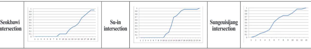
Accumulated observation probabilities of each intersection are shown in Fig. 4.
Since three intersections show similar characteristics, it is possible to combine field survey data into one set to get one accumulated empirical probability distribution. It is notable that this procedure may not appropriate to other cases
where study intersections are located different sites such as residential, commercial, industrial, and office areas, and having different characteristics. Obtained data sets for three intersections are shown in Table 5.
Seokbawi
intersection Su-in
intersection Sungeuisijang
intersection Fig. 4. Accumulated observation probabilities of study intersections
Number of
vehicle/cycle Observation
frequency Observation
probability (%) Accumulated observation
frequency
Accumulated observation
probability (%) Percentage difference (%)
0 0 0 0 0 -
1 1 0.9 1 0.9 0.9
2 2 1.8 3 2.7 1.8
3 1 0.9 4 3.6 0.9
4 2 1.8 6 5.4 1.8
5 6 5.4 12 10.8 5.4
6 3 2.7 15 13.5 2.7
7 2 1.8 17 15.3 1.8
8 2 1.8 19 17.1 1.8
9 2 1.8 21 18.9 1.8
10 6 5.4 27 24.3 5.4
11 4 3.6 31 27.9 3.6
12 8 7.2 39 35.1 7.2
13 31 27.9 70 63.1 27.9
14 3 2.7 73 65.8 2.7
15 6 5.4 79 71.2 5.4
16 4 3.6 83 74.8 3.6
17 3 2.7 86 77.5 2.7
18 2 1.8 88 79.3 1.8
19 0 0.0 88 79.3 0.0
20 1 0.9 89 80.2 0.9
21 21 18.9 110 99.1 18.9
22 0 0.0 110 99.1 0.0
23 1 0.9 111 100.0 0.9
Table 5. Data for diagraming empirical distributions
The accumulated empirical probability distribution is shown in Fig. 5.
Fig. 5 explains a lot. If you have enough budgets and spaces for left turn vehicles, you can provide the length of storage
lane containing 21 vehicles. However, if you have budget and space constraints, you may provide the length of storage lane containing only 12.5 vehicles satisfying only 50% of arriving vehicles. Once getting this type of accumulated empirical probability distribution diagram, planners and engineers can get help how to decide intersection design of left turn lanes.
4.2 The headways (S) at signalized intersections
We used UAV spatial images to measure left turn storage lengths of three intersections and headways. The UAV took photos from the top of the each site and imposed to an opened portal map service in public to precisely find left turn storage lengths. Details about headway and left turn storage length of each intersection are shown in Table 6. Buses were not observed during field survey in Su-in intersection.Fig. 5. Empirical left turn arrival distribution diagram in urban signalized commercial intersections
Classification
Left turn storage length (m)
(A)
Number of storage
vehicles (vehicle) (B)
Headway (m) (A/B)
Number of storage vehicles when mixing the
trucks (vehicle) Headway per vehicle (m)
Bus Large truck Bus Large
truck
Seokbawi intersection
172 26 6.61 24 13.2
Su-in intersection
135 18 9.56 - 16 - 19.1
Sungeuisijang intersection
110 14 7.86 12 15.68
Table 6. Storage lengths and headways of study intersections
Then, average headways for vehicle types are calculated as shown in Table 7 using UAV spatial images. Calculated average headways are 8.01 m for passenger cars, 14.44 m for buses, and 15.99 m for trucks, respectively.
Table 8 shows comparisons between investigated headways and vehicle lengths of design standard.
We found length differences of 2 m for passenger cars, 2.5 m for buses, and 4m for trucks, respectively. This result means that existing methodology calculates shorter left turn storage than needed lengths at fields and generates congestions.
It is helpful if we have information about the ratio of heavy vehicles in commercial areas in Incheon metropolitan city when using Table 8. After additional investigation, we found the ratio of heavy vehicles (buses and trucks). Among left turn vehicles, the ratios of heavy vehicles are found to be 4.45 %(buses occupy 2.83 % and trucks occupy 1.62 %, respectively) as shown in Table 9. This result can be used to calculate the left turn storage length at other similar intersections in commercial areas located in Incheon metropolitan city.
4.3 Storage length coefficient (α) at signalized intersections
The developed method may not need to use a storage length coefficient theoretically since it directly uses the number of arriving vehicles from an empirical distribution and the average headways. However, in real traffic situations, an uncertainty always inherits. Empirical distribution may change over time and the ratio of heavy vehicles can be changed. Vehicle types and specifications may also change over time.
Therefore, for sustainable design and safety purposes, flexibility should be provided at most of the design standard manuals.
From the literature review and other considerations, this study suggests to apply the values of 1.0 through 1.5 for the storage length coefficients as shown in Table 10.
Since 1.0 means only considering the minimum headway of arriving vehicles and 1.5 means providing maximum Classification Passenger car (m) Bus (m) Large truck (m)
Average
headway 8.01 14.44 15.99
Seokbawi
intersection 6.61 13.2 13.2
Su-in
intersection 9.56 - 19.1
Sungeuisijang
intersection 7.86 15.68 15.68
Table 7. Average headways of study intersections by vehicle types
Classification
Vehicle length by
design standards
Existing vehicle length (A)
Investigated average
headway (B) ︳A-B ︳
Passenger car 6.0 6.0 8.01 2.01
Bus 13.0
12.0 14.44 2.44
Large truck 16.7 15.99 3.99
Table 8. Comparing investigated average headways with vehicle length of design standards
Classification
Total number vehiclesof
Passenger (vehicle)car
(vehicle)Bus
Large truck (vehicle)
Rate (%) - 95.55 2.83 1.62
Sum 742 709 21 12
Seokbawi
intersection 296 277 18 1
Su-in
intersection 308 298 0 10
Sungeuisijang
intersection 138 134 3 1
Table 9. Rates of large trucks among left turn vehicles at urban commercial areas
Classification Coefficients of
signalized intersection Note Existing
coefficient 1.5 Suggested
coefficient 1.0~1.5 Standard is 1.0 When considering secure safety,
1.0 ~ 1.5 can be applied Table 10. Current and suggested coefficients for left turn
storage lengths
safety countermeasures considering uncertainty for design purposes at signalized intersections, fixing the value of coefficient at the level of design manual is not appropriate.
It is rather better for engineers to survey and determine the value of coefficient according to the environment of intersections considering.
4.4 Calculating relevant length of left turn storages at signalized intersection
Table 11 summarizes the developed calculating method for relevant length of left turn storages.
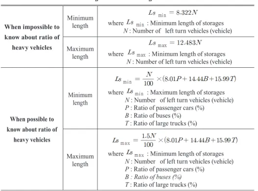
For more simplicity, Table 12 provides formulas for the cases whether we know the ratio of heavy vehicles or not.
5. Conclusions
This study developed a method for calculating relevant length of left turn storage lengths based on an empirical arriving distribution at signalized intersections in urban commercial areas in Incheon metropolitan city, South Korea.
This study show several results.
First, empirical distributions are developed for arriving distributions at signalized intersections in urban commercial areas to count the number of arriving vehicles. This empirical distribution method can be applied practically in any intersections where the number of arriving vehicles is concerned.
Secondly, this study suggests using an average headway using UAV spatial images instead of using an average length of vehicles for the waiting vehicles. Using an average headway of waiting vehicles can be more practical and efficient to accommodate characteristics of waiting vehicles.
Thirdly, the relevant range of storage length coefficients is designed to add flexibility of designing left turn storages instead of using some specified values that are not realistic in most cases.
Ls = α × N × S Ls : Length of left turn storage
α : Length coefficient (signalized intersection : 1.0~1.5) N : The number of left turn vehicles (vehicle) (arrival
vehicles per 1 cycle)
S : Average headway by vehicle types (m)
Table 11. Developed method for calculating length of left turn storages for signalized intersections in urban commercial areas
When impossible to know about ratio of
heavy vehicles
Minimum
length where : Minimum length of storages N : Number of left turn vehicles (vehicle) Maximum
length where : Minimum length of storages N : Number of left turn vehicles (vehicle)
When possible to know about ratio of
heavy vehicles
Minimum length
where : Maximum length of storages N : Number of left turn vehicles (vehicle) P : Ratio of passenger cars (%)
B : Ratio of buses (%) T : Ratio of large trucks (%)
Maximum length
where : Minimum length of storages N : Number of left turn vehicles (vehicle) P : Ratio of passenger cars (%) B : Ratio of buses (%)
T : Ratio of large trucks (%)
Table 12. Formula for length of left turn storages in urban commercial area
Fourthly, formulas are developed to calculate relevant length of left turn storages when impossible to know, and possible to know ratio of heavy vehicles at urban commercial areas based on vehicle types.
By applying the develop method and values, rear-end collisions caused from irrelevant left turn storage lengths can be decreased and more efficient signalized intersection operation can be accomplished.
Acknowledgments
This work was supported by the Incheon National University Research Grant in 2013.
References
AASHTO (2011), A Policy on Geometric Design of Highways and Streets, Transportation Officials, USA. pp. 1-8.
Do, C. (2005), Transportation Engineering Principles(1) 2nd Edition, Chungmoongak, Seoul, Gangnan-gu. Republic of Korea, pp. 67, 90-91.
Incheon Metropolitan City (2009), City planning complete map, Incheon Metropolitan City, http://www.incheon.
go.kr/index.do/ (last date accessed: 10 May 2018).
ITE (2008), Urban Street GEOMETRIC DESIGN HAND- BOOK, Institute of Transportation Engineers, Washington, D.C., USA. pp. 199-200.
JRA (2005), Rules of Road Guideline for Commentary and Management, Japan Road Association, Ministry of Land and Transportation, Japan.
Kelton, W.D. and Law, A.M. (2007), Simulation Modeling &
Analysys Fourth Edition, McGraw-Hill, Inc., New York, pp. 301-312.
Kim, J. L. (2002), A study on the Capacity Calibration of Left Turn Bay to Signalized Intersection, Ph.D. dissertation, Keimyung University, Daegu, Korea, 144p.
KSCE (2009), Rules of Road Structure and Facility Standards, Korean Society of Civil Engineers, Republic of Korea.
Lee, S. (2009), A Study of Arrival Distribution of Left- Turning Vehicles at Signalized Intersections, Master's thesis, Yonsei University, Seoul, Korea, 60p.
Yekhshatyan, L. and Schnell, T. (2008), Turn Lane Lengths for Various Speed Roads and Evaluation of Determining Criteria, MN/RC 2008-14, MNDOT, Minnesota, pp. 8-14 KoROAD (2015), Traffic accident analysis system(2015),
TAAS, http:// taas.koroad.or.kr/ (last date accessed: 10 May 2018), Korea Road Traffic Authority, Republic of Korea.
Fitzpatrick, K., Wooldridge, M. D., & Blaschke, J. D. (2005), Urban Intersection Design Guide, Product 0-4365-P2 Vol.
1, TxDOT, Texas, pp. 4-6.
Qi, Y., Yu, L., Azimi, M., and Guo, L. (2007), Determination of Storage Lengths of Left-Turn Lanes at Signalized Intersections, Transportation Research Record, Vol. 2023, pp. 102-111.