Reusable Network Model using a Modified Hybrid Genetic Algorithm in an Optimal Inventory Management Environment

* Corresponding Author: [email protected]

Manuscript received July 03, 2019 / revised July 23 ,2019 / accepted July 25, 2019

1) 동의대학교 경영학부 회계학전공, 제 1저자

1. Introduction

Logistics activities consist of numerous

최적 재고관리환경에서 개량형 하이브리드 유전알고리즘을 이용한 재사용 네트워크 모델

(Reusable Network Model using a Modified Hybrid Genetic Algorithm in an Optimal Inventory Management Environment)

이 정 은

(JeongEun Lee)

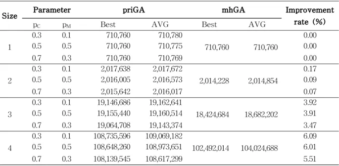
요 약 본 연구에서는 재사용 가능한 제품을 대상으로 순방향물류(Forward logistics)에서 부터 역방향물류(Reverse logistics)에 이르기까지 전체 물류비용과 수요와 회수에 따른 제조업자에서의 재 고관리, 재사용을 위한 과정에서 발생하는 청소공정비용 및 폐기비용을 고려한 재사용 네트워크 모델 (Reusable network model)을 제안한다. 제안 모델의 유효성을 검증하기 위하여 최적화 기법 중 하나 인 유전자 알고리즘(Genetic algorithm: GA)을 이용한다. 파라미터가 해(Solution)에 미치는 영향을 알 아보기 위해서 세 가지 파라미터 조건에서 우선 순위형 GA(Priority-based GA: priGA)와, 각 세대 (Generation)마다 파라미터가 조정되는 개량형 하이브리드 GA(Modified hybrid genetic algorithm:

mhGA)를 사이즈가 다른 4가지 예제에 적용하여 시뮬레이션을 실시한다.

핵심주제어: 재사용 로지스틱스 모델, 개량형 하이브리드 유전알고리즘, 우선순위형 유전알고리즘, 재고관리, 역물류

Abstract The term ‘re-use’ here signifies the re-use of end-of-life products without changing their form after they have been thoroughly inspected and cleaned. In the re-use network model, the distributor determines the product order quantity on the network through which new products are received from the suppliers or products are supplied to the customers through re-use of the recovered products. In this paper, we propose a reusable network model for reusable products that considers the total logistics cost from the forward logistics to the reverse logistics. We also propose a reusable network model that considers the processing and disposal costs for reuse in an optimal inventory management environment. The authors employe Genetic Algorithm (GA), which is one of the optimization techniques, to verify the validity of the proposed model. And in order to investigate the effect of the parameters on the solution, the priority-based GA (priGA) under three different parameters and the modified Hybrid GA (mhGA), in which parameters are adjusted for each generation, were applied to four examples with varying sizes in the simulation.

Keywords: Reusable logistics model, mhGA(modified hybrid genetic algorithm), priGA(priority-based genetic algorithm), Inventory management, Reverse logistics

activities ranging from demand forecasting to customer ordering, raw material purchasing, material handling and collection, including transportation and inventory management. Of these, the most noteworthy category is reverse logistics. Reverse logistics refers to the activities related to the return of the product delivered to the customer through the forward logistics activity to the producer, with growing importance in the logistics activity. As the amount of the material transferred from the producer to the customer increases, the amount of the collected return material is increased as well. In other words, the scale of reverse logistics is continuously increasing including such cases as when the return is made due to the customer's remorse or product abnormality after the product was delivered to the customer through forward logistic, or when the end-of-life products are recovered, on in the case of waste disposal.

Therefore, the importance of reverse logistics activities is increasing more than ever considering the economic and environmental viewpoints.

Murphy and Poist(2007) clarified the scope by defining reverse logistics as the movement of the product from the consumer to the producer on the distribution channel. However, they redefined the reverse logistics afterwards not simply as a movement of goods but as a suite of activities covering the entire range including return of goods, reduction of resources, reproduction, substitution of resources, re-use of goods, waste disposal, reprocessing, repair, and reproduction.

Looking at the economic aspects of recovery logistics, it is possible to reduce the amount of resources to be disposed of and shave off processing cost by reusing products, reproducing and recycling parts. In addition, when the supply of raw materials is

irregular, it can also serve as an efficient source of supply by utilizing collected resources. As a result, the producers can maximize the efficiency of the work, secure the supply stability, and reduce the purchase cost by using the recovered resources efficiently, there realizing sweeping performance across the board(Yu, 2007). The collection policy of reverse logistics is used as a means of promoting sales and publicizing the offer. And it is also directly connected with corporate image management.

In addition, timely post-sale reverse logistics activities have a direct impact on customer satisfaction of services, further leading to product backorders and corporate profitability.

Turning to the environmental aspects of recovery logistics, the European Union adopted the Waste Electrical and Electronic Equipment (WEEE) and the End of Life Vehicle (ELV) convention to directly regulate the disposal of batteries, tires, or hazardous wastes(The EU’s Approach to Waste Management, 2019).

Such reverse logistics can be divided into three types of networks: re-use, remanufacturing, and recycling(Kim et al., 2004).

Re-use here signifies the re-use of end-of-life products without changing their form after they have been thoroughly inspected and cleaned. Sitting in the intermediate position of 3R (Reduce, Re-use, Recycle), re-use is a keyword for forming a closed-loop society in which environment and economy can coexist harmoniously.

Typical examples of re-use are bin bottles,

containers, and pallets. By recycling empty

bottle containers and using them repeatedly,

environmental burdens such as waste and

CO

can be reduced. Kroon and Vrijens(1995)

proposed a quantitative model of recovery

logistics considering the actual cases of logistics companies in the environment of re-use of packaging containers. Fleischmann et al.(1997) investigated the logistics network considering product re-use practices in various industries and proposed a classification system of product re-use networks as compared to the traditional logistics network.

Jayaraman et al.(1999) proposed a mathematical model of reverse distribution in multi-item problems with general supply and demand, and conducted a study on reverse distribution.

Pishvaee et al.(2010) presented a mathematical model that minimizes transportation costs and fixed costs in reverse logistics, and the n derived value via simulated annealing which is a stochastic heuristic approach.

This paper is differentiated in that it proposed a network model that integrates the entire transportation flow from the general logistics to the whole transportation flow of the collection and logistics, the inventory management and the re-use process, whereas existing papers dealt with recovery logistics, its methodology, and the use and management of recovery vessels.

This paper proposes an improved model that calculates the total logistics cost, the cleaning process cost, and the disposal cost through the optimization methodology and integrates optimal inventory management according to demand and recovery.

The main purpose of this study is to establish a mathematical model of optimization for forward and reverse logistics that considers the minimization of the total cost, using the modified hybrid genetic algorithm (mhGA) model.

This paper differs from the other studies in the literature in that it simultaneously considers the cost in the forward and reverse logistics field (forward logistics: inventory and purchase; reverse logistics: retuning, cleaning, and disposal) and an effective inventory and order system in a multi-period.

This paper is organized as follows. In section 2, the problem concerning the design of the forward and reverse logistics network is defined more concretely, and the mathematical model of such network is introduced. In section 3, priority-based encoding genetic algorithm(priGA) and modified hybrid genetic algorithm(mhGA) are explained to solve the problem. In section 4, the results of the numerical experiments that were conducted in the study are presented to demonstrate the efficiency of the proposed method. Finally, in section 5, the concluding remarks and future research directions are discussed.

2. Problem Definition

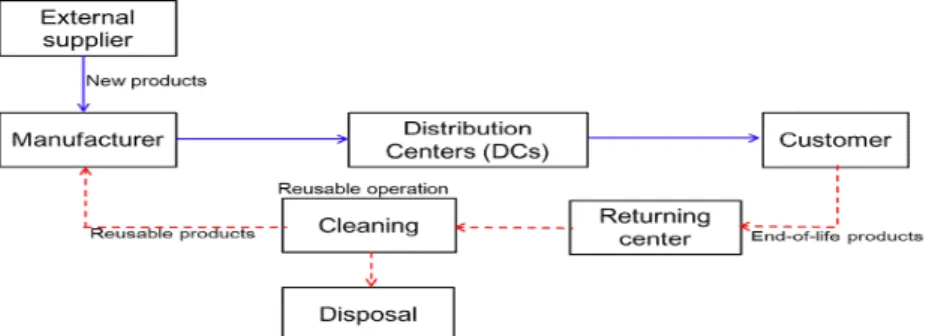
Fig. 1 Reusable Logistics Model

2.1 Model Description

In the reusable network model, the distributor determines the product order quantity on the network through which new products are received from the suppliers or products are supplied to the customers through re-use of the recovered products(Lee, 2012).

This paper considers the forward and reverse logistics network design problem with the concepts of transportation cost and inventory.

In a planning horizon, a mathematical model is established to determine the amount of each product, which should be shipped between two echelons in each period of time.

Besides, the objective function is to minimize the total cost of the forward and reverse logistics, including the inventory and purchase costs.

In the reverse logistics, it is more difficult to meet the customer's desired delivery date than general forward logistics because the amount of recovered products is uncertain.

Thus, potential loss of customers due to complaints about the delay can be prevented by minimizing the waiting time.

As shown in Fig. 1, the forward and reverse logistics network consists of the supplier, manufacturer, DCs, customer zones, returning center, processing center, and disposal center. The general forward and reverse logistics recover the products to the customers.

2.2 Assumptions

We consider the single product case of the reverse and forward logistics problem considering planning horizons, and give some assumptions, based on which we formulate this problem.

- The disposal rate of used products shipped to the processing center is rounded up to 0.1%.

- The maximum capacity of each center is known.

- The customer's location is known.

- Only one product is treated in the forward and reverse logistics network model.

- The inventory factor exists over the finite planning horizons.

- The requirement by the manufacturer and the quantity of collected products are known in advance.

2.3 Notations

1) Indices

i : supplier index ( i ∈ I ) j : manufacturer index ( j ∈ J ) k : distribution center index ( k ∈ K ) l : customer index ( l ∈ L )

m : returning center index ( m ∈ M ) n : cleaning center index ( n ∈ N ) p : disposal center index ( p =∈ P ) t : time period index ( t ∈ T )

2) Parameters

a

: capacity of supplier i a

: capacity of manufacturer j a

: capacity of distribution center k a

: capacity of returning center m a

: capacity of cleaning center n a

: capacity of disposal center p

r

( t ): amount of end-of-life product recovered to returning center m in period t

d

( t ): demand on manufacturer j in period t c

: unit cost of transportation from supplier i

to manufacturer j

c

: unit cost of transportation from manufacturer j to distribution center k

c

: unit cost of transportation from distribution

center k to customer l

c

: unit cost of transportation from customer l to returning center m

c

: unit cost of transportation from returning center m to cleaning center n

c

: unit cost of transportation from cleaning center n to manufacturer j

c

: unit cost of transportation from cleaning center n to disposal center p

c

: unit holding cost of inventory per period at manufacturer j

c

: unit purchase cost at supplier I

c

: unit processing cost at cleaning center n c

: unit disposal cost at disposal center p r

: disposal rate

3) Decision Variables

x

( t ): amount shipped from supplier i to manufacturer j in period t

x

( t ): amount shipped from manufacturer j to distribution center k j in period t x

( t ): amount shipped from distribution center

k j to customer l in period t

x

( t ): amount shipped from customer l to returning center m in period t

x

( t ): amount shipped from returning center m to cleaning center n in period t x

( t ): amount shipped from cleaning center n

to manufacturer j in period t

x

( t ): amount shipped from cleaning center n to disposal center p in period t

y

( t ): inventory amount delivered to manufacturer j in period t

y

( t ): purchase amount delivered to supplier i in period t

y

( t ): processing amount delivered to cleaning center n in period t

y

( t ): disposal amount delivered to disposal center p in period t

2.4 Model Formulation

In this paper, reverse logistics and forward

logistics are considered at the same time, and detailed costs are summarized as follows.

Minimize = forward logistics + reverse logistics Forward logistics costs = transportation cost +

inventory cost + purchase cost

Reverse logistics costs = transportation cost + processing cost + disposal cost

1) Objective Function

The objective function is to minimize the total cost of the forward and reverse logistics model of reuse recovery considering inventory, processing, purchase, and disposal, and the transportation costs from the supplier to the customer and manufacturer.

min 





  







  





  



__ 



  





  



__ 



  





  



__

_{  }



















_{  }









2) Subject to

_^  _^  _^   _^ ∀∈ ∈ 

_^_^ ≥ _^_^  _^_^ ∀∈ ∈ 

  





_^ 



  





  



_^ ∀ ∈ 

  





_ ≤ _ ∀ ∈ ∈ 

  





_ _   _ ≤ _ ∀∈ ∈ 

  





_ ≤ _ ∀ ∈ ∈ 

  





_ ≤ _ ∀ ∈ ∈ 

  





_ ≤ _ ∀ ∈ ∈ 

_ _ ≥ _ ∀ ∈ ∈ 

_ _ _ _ _ _

_ _ ≥ 

∀ ∈ ∈ ∈ ∈ ∈ ∈ ∈ ∈ 

Constraint (2) shows inventory amount of manufacturer. Constraint (3) represents principle of matching costs with revenues. Constraint (4) represents disposal costs. Constraints (5) to (8) represent capacities of manufacturer, distribution center, cleaning center, disposal center. Constraint (9) shows the recovered amount of end-of-life products. Constraint (10) represents demand constraint. Constraint (11) is non-negativity of decision variables.

The problem of reusable network is one of the NP-hard problems. The problem of mixed integer programming with a relatively small number of integer variables can be solved within practical time by using conventional optimizing software. In the scale of the problem to be solved in this paper, however, computation time or memory used increases exponentially, making it impossible to apply.

Therefore, the approximate optimal solution will be calculated by using the genetic algorithm described in Section 3 as a solution of this problem.

3. Solution Approach

Numerous heuristic algorithms have been developed along with optimal solutions for dealing with the network optimization model modeled in Section 2. Therefore, the authors used the hGA proposed by Gen et al.(2008).

FLC(Fuzzy logic controller) has the advantage of automatically adjusting the balance between exploitation and exploitation based on

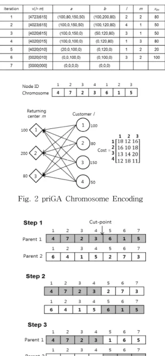
Table 1 priGA Decoding

Fig. 2 priGA Chromosome Encoding

Fig. 3 Weight Mapping Crossover

Fig. 4 Swap Mutation

changes in the average fitness of current and last generation.

Genetic algorithms are one of the techniques for probabilistic search and learning and optimization. Just as the survival of the fittest is determined by the relationship between the individual and the environment surrounding it, the fitness of specific point is determined by the extent to which the point in the search space of the genetic algorithm matches the given problem. Probability is considered to be the dominant factor through the whole process of genetic algorithm with the performance of the algorithm determined by the determination of its specific value.

Therefore, the algorithm has a characteristic of stochastic search, which is influenced by the probability of genetic algorithm, and also searches for direction that we can move to the point we want without the help of information such as slope. To find the optimal solution, the algorithm generates a population of randomly extracted solutions from the solution set. This is called an initial population, and the population is searched repeatedly through selection, crossover and mutation. In this group of individuals, the algorithm selects the appropriate object for the given problem and makes the next generation (offspring), and the search is ended when there is something we want to find in that group of individuals, or if it exceeds the number of generations that we set in advance through several generations of repetition (Gen and Cheng, 2000).

3.1 Priority-based Genetic Algorithm (priGA)

As shown in Fig. 2, priGA generates a chromosome having a total length (4+3) of the customer L and the collection center M . The numbers on each gene represent

priorities, and the initial values of the priority start from the number of chromosome lengths ( L + M =7) and are repeated until they are randomly assigned to all genes. In addition, the customer and return center numbers represent the respective capacity, and the cost represents the shipping cost of the collection center from the customer.

In Fig. 2, the highest priority (7) is given to the chromosome and Customer 2 has the lowest cost when transporting to collection center 2. Since the capacity of Customer 2 is 80 and the number of the collection center 2 is 200, the capacity deliverable from the customer to the collection center is 80.

Therefore, Customer 2 is transported to collection center 2, thereby making customer capacity to 0, while collection center 1 having the next priority is selected, and transportation quantity is determined in this manner. Table 1 shows the calculation procedure.

3.2 Genetic Operators

1) Crossover Operator

For the WMX (Weight Mapping Crossover) intersection, the cut point is set at random as shown in Fig. 3 and the right chromosome part of the cut point is replaced. The replaced right section shall be lined up from the lowest number before replacing each number with a pair of numbers to create a child chromosome (Gen et al., 2008).

2) Mutation Operator

For Swap Mutation, randomly select pairs

of genes to be exchanged in the gene (for

example, 2 and 5), and exchange the selected

two genes as shown in Fig. 4 (Gen et al.,

2008).

3.3 Hybrid Genetic Algorithm

In general, genetic algorithms fix genetic strategy parameters and similarly reproduce the evolutionary process based on those values. In this method, however, the intersection or mutation always occurs at the same probability, and the diversity required for the evolution process is lost. If the GA parameters can be appropriately adjusted to the situation of the group, not only the quality of the solution is improved, but the calculation time of the simulation is expected to be shortened. Increasing the mutation rate, which is a parameter of genetic manipulation, broadens the search range, while decreasing the mutation rate increases the accuracy of local search. It is possible to increase the search speed and accuracy of the solution by appropriately adjusting the mutation rate. The mhGA used the chromosome representation of priGA and employed FLC where the parameters are adjusted appropriately for each generation, and the optimal situation is

created by searching the optimal solution (Lin et al., 2009).

The method of obtaining the cross rates and the mutation rate using the FLC is as follows (Gen and Cheng, 2000; Lin and Gen, 2009).

① The change in the average evaluation value of the current and previous generation groups is calculated by the following equation.

∆

   

   

  

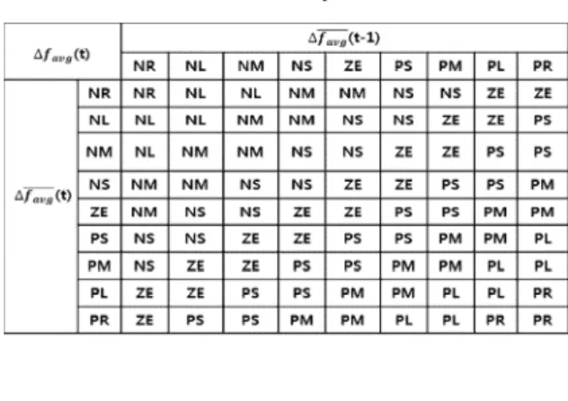
② The control operation corresponding to the change (increase or decrease) of the average evaluation value of the current generation and the previous generation is determined using Table 2.

③ The variation of the crossover rate and the mutation rate corresponding to the result of ② is obtained using Table 3.

And then, the amount of change in the crossover rate and the mutation rate is calculated by the following equation.

The amount of change in the crossover rate

∆

  

·    

where r

is a adaptation coefficient.

The amount of change in the mutation rate

∆

  

·    

where r

is a adaptation coefficient.

④ Use the following equation to determine the crossover rate and the mutation rate for the next generation.

_    _ ∆_

_    _  ∆_

where λ is a forgetting factor.

Fig. 5 shows the calculation flow of mhGA.

Fig. 5 Flow Chart of mdGA

4. Computation Results

To evaluate the performance of mhGA for solving the forward and reverse logistics network design problem, this problem was compared with priGA. The reason that priGA was selected as a basis of comparison was its similarity to mhGA in the use of a priority-based encoding method.

4.1 Data Generation

The data for these problems randomly considered by some researchers were generated, as shown in Table 4. The data in the test problems, such as the transportation cost, product demand, and the capacities of the manufacturer, DCs, returning centers, processing center, and disposal center were also randomly generated to provide realistic scenarios.

The effectiveness of the FLC proposed by Eiben et al.(1999) was investigated. FLC is a heuristic rule for controlling the mutation rate.

Lin et al.[12] explained that FLC is dynamically regulated by using a linear function of the number of generations using the mutation rate p

. All the test problems were solved on an Intel Core i3-3220 CPU, a 3.30GHz clock pulse with 4GB memory.

4.2 Numerical Results

To validate the proposed model and mhGA, we compared priGA and mhGA in Table 3.

An experiment was performed by 20 times each and shows the result for Table 5.

In general, the result of GA decreased with increasing the problem size means that we have to increase GA parameter settings (Lee et al., 2008).

In order to examine the effect of the parameters on the solution and to verify the performance of the proposed mhGA, the WMX crossing rate and the exchange mutation rate were set at (0.3, 0.1) and (0.5, 0.5), respectively. The simulation was performed by applying the mhGA to the four different numerical examples of different sizes.

no. j l l t popS* Max.G*

1 1 10 1 2 100 500

2 2 20 2 4 100 500

3 3 30 3 4 100 500

4 4 40 4 4 100 500

* popS: Population size

* Max. G. : Max. generation Table 4 Experiment Data

Table 2 Fuzzy Table

Table 3 Look-up Table

As a result, the minimum cost solution was obtained under the parameter condition of (0.7, 0.3) in priGA, while the minimum cost suboptimal solution was obtained in the case of mhGA in the comparison of priGA and mhGA. As the size of the case example increases, the quality of the solution of mhGA is better than that of priGA.

Fig. 6 shows the convergence behavior of the four methods for test problem 1. The value of the solution was not changed after 350 generation. Because evolution is early, a solution provided by mhGA may converge in a local minimum, but there does not seem to be the problem for the moment. The mhGA gives a smaller best value than priGA.

The effectiveness of the proposed FLC was thereby proven. The modified Hybrid GA provides an optimal solution for the optimization methods of the reverse and forward logistics model by adjusting parameter appropriately in each generation.

5. Conclusions

In this study, the authors considered the forward logistics and reverse logistics in the reusable logistics model to calculate the total transportation cost, the cleaning process cost and the disposal cost. We also proposed an improved model that integrates optimal inventory management according to demand and recovery.

The proposed reusable network model is one of the NP-hard problems. This is a more realistic TP model, and factory-produced products are reusable products that are

Fig. 6 Convergence Behaviors of the Different Approaches in Problem 1 (0.7, 0.3)

Size Parameter priGA mhGA Improvement

rate (%)

p

p

Best AVG Best AVG

1

0.3 0.1 710,760 710,780

710,760 710,760

0.00

0.5 0.5 710,760 710,775 0.00

0.7 0.3 710,760 710,769 0.00

2

0.3 0.1 2,017,638 2,017,672

2,014,228 2,014,854

0.17

0.5 0.5 2,016,005 2,016,573 0.09

0.7 0.3 2,015,642 2,016,017 0.07

3

0.3 0.1 19,146,686 19,162,641

18,424,684 18,682,202

3.92

0.5 0.5 19,155,440 19,160,514 3.91

0.7 0.3 19,064,708 19,143,374 3.47

4

0.3 0.1 108,735,596 109,069,182

102,492,014 104,024,688

6.09

0.5 0.5 108,648,260 108,973,651 6.01

0.7 0.3 108,139,545 108,617,299 5.51

Table 5 Results of the Simulation

transported to the end consumer, then retrieved, processed and re-used. Also, the mathematical model is nonlinear making it difficult to find the most suitable solution with general LP software. Therefore, the suboptimal solution was obtained using the genetic algorithm as a solution to this problem.

In order to verify the usefulness of the proposed algorithm, we compared the priGA and mhGA. As a result, the least cost solution was obtained under the parameter condition of (0.7, 0.3) in priGA, while in the comparison between priGA and mhGA, the suboptimal solution of the least cost was obtained in mhGA. It was also confirmed that as the size of the case increases, the improvement rate of the quality of mhGA is better than that of priGA.

Future tasks would include: (1) Apply the proposed method to the actual data in order to verify the validity and efficiency of the proposed method, and (2) Compare the simulated annealing and Tabu Search which is an optimization technique.

References

Eiben, A. E., Hinterding, R. and Michalewicz, Z. (1999). Parameter Control in Evolutionary Algorithms, IEEE Transactions on Evolutionary Computation , 3(2), 124-141.

Fleischmann, M., Bloemhof-Ruwaard, J. and Dekker, R. (1997). Quantitative Models for Reverse Logistics: a Review, European Journal of Operational Research , 103(1), 1-17.

Gen, M. and Cheng, R. (2000). Genetic Algorithms and Engineering Optimization , New York, John Wiley & Sons.

Gen, M., Cheng, R. and Lin, L. (2008).

Network Models and Optimization:

Multiobjective Genetic Algorithm Approach , London, Springer.

Jayaraman, V., Guide, V. D. R. and Srivastava, R. A. (1999). A Closed Loop Logistics Model for Remanufacturing, J ournal of the Operational Research Society , 50(5), 497-508.

Kim, J. Y., Kim, K. B. and Cheong, B. J.

(2004). Recycle, Recycle Logistics Network Model considering Reuse, Recycle and Reproduction, Fall Conference of Korea Industrial Engineering Association , Nov.

13th, Seoul.

Kroon, L. and Vrijens, G. (1995). Returnable Containers: an Example of Reverse Logistics, International J ournal of Physical Distribution and Logistics Management, 25(2), 56-68.

Lee, J. E. (2012). Modeling and Optimization of Reverse Logistics for Reuse and Remanufacture , Ph. D. Thesis, Waseda University, Japan.

Lee, J. E., Gen, M. and Rhee, K. G. (2008).

Network Model and Optimization of Reverse Logistics by Hybrid Genetic Algorithm, Computers and Industrial Engineering , 56(3), 951-964.

Lin, L., Gen, M. and Xang, X. (2009).

Integrated Multistage Logistics Network Design by using Hybrid Evolutionary Algorithm, Computer and Industrial Engineering, 56(3), 854-873.

Lin, L. and Gen, M. (2009). Auto-turning Strategy for Evolutionary Algorithms:

Balancing between Explorations and Exploitation, Soft Computing, 13(2), 157-168.

Murphy, P. R. and Poist, R. F. (2007). Skill Requirements of Senior-level Logisticians: a Longitudinal Assessment, Supply Chain Management: An International Journal, 12(6), 423-431.

Pishvaee, M. S., Farahani, R. Z. and Dullaert,

W. (2010). A Memetic Algorithm for Bi-objective Integrated Forward/reverse Logistics Network Design, Computer and Operations Research , 37(6), 1100-1112.

The EU’s Approach to Waste Management, http://ec.europa.eu/environment/waste/weee/

(Accessed on June 28th, 2019)

Yu, S. C. (2007). Development of Evaluation Model for Collected Logistics Companies and Establishment of Purchasing Strategy Considering Recovery Product Characteristics , Ph. D. Thesis, Graduate School of Korea University, Korea.

이 정 은 (JeongEun Lee)

∙정회원

∙동의대학교 회계학과 경영학사

∙동의대학교 회계학과 경영석사

∙와세다대학교 정보생산시스템 연구과 공학박사

∙동의대학교 상경대학 경영학부 회계학전공 부교수

∙관심분야 : 최적화, 회계정보시스템