Partial Inverse Traveling Salesman Problems on the Line

JKSCI

Partial Inverse Traveling Salesman Problems on the Line

1)

Yerim Chung*, Myoung-Ju Park**

*Professor, School of Business, Yonsei University, Seoul, Korea

**Professor, Dept. of Industrial and Management Systems Engineering, Kyung Hee University, Youngin, Korea [Abstract]

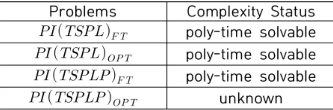
The partial inverse optimization problem is an interesting variant of the inverse optimization problem in which the given instance of an optimization problem need to be modified so that a prescribed partial solution can constitute a part of an optimal solution in the modified instance. In this paper, we consider the traveling salesman problem defined on the line ( on the line) which has many applications such as item delivery systems, the collection of objects from storage shelves, and so on. It is worth studying the partial inverse  on the line, defined as follows. We are given  requests on the line, and a sequence of  requests that need to be served consecutively. Each request has a specific position on the real line and should be served by the server traveling on the line. The task is to modify as little as possible the position vector associated with  requests so that the prescribed sequence can constitute a part of the optimal solution (minimum Hamiltonian cycle) of  on the line. In this paper, we show that the partial inverse  on the line and its variant can be solved in polynomial time when the sever is equiped with a specific internal algorithm Forward Trip or with a general optimal algorithm.

▸Key words: Inverse Optimization, Partial Inverse Problem, Traveling Salesman Problem, Poly-time Algorithm, TSP on the Line

[요 약]

부분역최적화는 역최적화의 흥미로운 변형으로, 주어진 최적화문제와 그 문제의 부분해가 주어

지면 이 부분해가 최적해에 포함되도록 문제를 최소한으로 수정하는 문제이다 . 이 논문은 라인

위에서 정의되는 순환외판원문제()를 다루는데, 이는 배달시스템, 창고 선반에서 물건을 수집 하는 것, 등의 많은 응용을 가진다. 라인 위에서 위치하는 개의 일이 주어지고 이 중 연속적으 로 처리해야하는 일 개가 부분적으로 주어진다. 각각의 일은 라인 위의 특정 장소에 위치하고 라인을 움직이는 서버에 의해 처리되어야 한다. 우리의 임무는 개의 일이 최적해에서 연속적으 로 처리되도록 개의 일의 위치를 라인 위에서 최소한으로 조정하는 것이다. 이 논문에서 이 문 제와 이 문제의 다양한 변종을 다항시간 내에 푸는 알고리즘을 개발한다 . 구체적으로, 서버가 특 정한

용하는 경우에 대한 부분역최적화를 다룬다.

▸주제어: 역최적화, 부분역최적화, 순환외판원문제, 다항알고리즘, 라인 위에서의 TSP

∙First Author: Yerim Chung, Corresponding Author: Myoung-Ju Park

*Yerim Chung ([email protected]), School of Business, Yonsei University

**Myoung-Ju Park ([email protected]), Dept. of Industrial and Management Systems Engineering, Kyung Hee University

∙Received: 2019. 10. 10, Revised: 2019. 11. 05, Accepted: 2019. 11. 05.

Copyright ⓒ 2019 The Korea Society of Computer and Information http://www.ksci.re.kr pISSN:1598-849X | eISSN:2383-9945

I. Introduction

Given a problem, we usually aim to find the optimal solution. However, it is not trivial to find the best solution, especially in the case where the given problem is intrinsically hard to solve. The traveling salesman problem( for short) is the one of such problems.

On the other hand, it is relatively easy to get a feasible solution, even for the hard optimization problems. The inverse optimization problem is defined with the goal of making the prescribed feasible solution optimal in the new instance rather than finding an optimal solution[1-3]. The inverse optimization has been studied for many combinatorial optimization problem such as the shortest path problem, the minimum spanning tree problem, the maximum independent set problem, the minimum graph coloring problem,  , and so on[4-13].

The partial inverse optimization problem is an interesting variant of the inverse optimization problem in which a partial solution is given instead of a whole feasible solution. The objective is to modify the least possible the instance of the problem so that the prescribed partial solution becomes a part of the optimal solution in the modified instance. The partial inverse problem has been studied for the assignment problem, minimum cut problem, the shortest path problem, , and so on[14-16].

For  , the inverse optimization and the partial inverse optimization problems have been studied by [8, 17]. In [8], the authors show that the inverse  against the closest neighbor algorithm can be solved in polynomial time, and the problem against 2-opt is NP-hard when the edge length are restricted to 1 or 2. In [17], the partial inverse  is shown to be NP-hard against both Closest Neighbor, and 2-opt.

In this paper, we study the partial inverse traveling salesman problem defined on a special metric space, the real line. While  is the one of the most well-known NP-hard problem[18], 

on the line becomes trivial. For  on the line space, the inverse problem is studied by [8] and it is shown that the inverse traveling salesman problem can be solved in  log time. However, the partial inverse problem for  on the line has not been studied yet.

In practice,  on the line (, for short) has many applications such as robotic welding, item delivery systems, and the collection of objects from storage shelves, and so on. In practice, we may have some partial solution for . It can be a list of objects that need to be collected in order, or a list of items that need to be delivered consecutively. It is worth studying its partial inverse version where the given partial solution can become a part of an optimal solution for

.

The partial inverse traveling salesman problem on the line is defined as follows and we denote it by

  .

We deal with two versions of partial inverse traveling salesman problem on the line. The one is defined with a partial solution of  which is a subsequence of requests that need to be served consecutively. The other is defined with a subset of requests with a specific prescribed order(e.g., precedence conditions). We denote the former by

   and the latter   .

Definition 1.  .

Given  requests on the horizontal line, and a sequence of  requests,   is to modify as little as possible the positions of some requests on the line so that the given sequence of  requests can be can be a part of the optimal 

-solution.

Definition 2.   .

Given  requests on the horizontal line, and  requests with precedence conditions in the prescribed order,   is to modify as little as possible the positions of some requests on the line so that the given  requests can be served in the prescribed order by the server in the optimal

-solution, while satisfying the precedence conditions between requests.

This paper is organized as follows: In Section II, we introduce the partial inverse traveling salesman problem on the line against a specific algorithm. In Section III, we discuss the polynomial time solvability of the partial inverse traveling salesman problem on the line against any optimal algorithm.

We consider in Section IV the partial inverse traveling salesman problem on the line with precedence conditions, and discuss the relation with the minimum cost flow problem. We then conclude the paper.

II. Partial Inverse Traveling Salesman Problems on the Line against a

Specific Algorithm

Let us consider the partial inverse traveling salesman problem on the line against a specific algorithm  for  , denoted by   _ . In [4], the authors introduced the inverse problem against a specific algorithm. The objective is to determine a new instance at a minimum cost (with minimum modification) such that the given feasible solution can be selected as a best solution when applying the algorithm.

In    _ , we are given  requests dispersed along a horizontal line space, and  requests that need to be served consecutively by the server. The server decides the order to serve the requests by using its specific internal algorithm

 in order to minimize the makespan, i.e., the time until all requests have been served. It may often happen that the given  requests cannot be visited in the prescribed sequential order in the optimal tour returned by the algorithm. The objective of

    is to modify as little as possible the positions of some requests on the line in such a way that the given sequence  requests can constitute a part of the best solution returned by

 .

As a specific algorithm for solving  on the line space, we consider the greedy algorithm, called Forward Trip (, for short).  starts the trip from the leftmost request on the line and satisfies all the requests in its forward trip; no request can be served on the way back. It is clear that  is an optimal algorithm for  on the line (

for short).

Note that an instance of  can be described as a position vector    _ ⋯ _  of  requests on the real line space. Then   _{ } can be defined as follows.

Definition. Given a position vector    _ ⋯ _  of  requests on the real line and a sequence

 _   _ ⋯  _ of  requests,   _{ } is to find a new position vector    _ ⋯  _  such that the given sequence can be a part of the optimal tour returned by  in the new instance, and the total deviation ║  ║ _ between the original and new position vectors becomes minimum under the

 _ -norm.

Focusing on the given  requests that need to be served consecutively (without preemption), we consider the following sets of indices. We denote by

   ^{∈    ⋯   }  ≤  _  the indices of the

requests located on the left-hand side with respect

to the request  _ , and denote by

   ^{∈     ⋯   }  ≥  _  the indices of the requests originally located on the right-hand side with respect to the request  _ .

Then, one can rewrite   _{ } as follows.

 _  min 

  



 _   _  subject to

max _{∈ }  _ ≤  _ ≤  _ ≤⋯≤  _ ≤ min _{∈ }  _

Proposition 1.   _ has an optimal solution such that  _ ≤  _ if  _ ≤  _ for any

 ∈    ⋯  .

Proof. Let    _ ⋯  _  be an optimal solution of   _{ } . Assume that for some

 ∈    ⋯  , we have  _ ≤  _ and  _ ≥  _ . Now we consider another feasible solution ′ such that ′ _   _  ′ _   _ and ′ _   _ for any  ≠  .

It is easy to see that ′ is at least as good as the given optimal solution . By repeating this, we can obtain an optimal solution for    _{ } such that  _ ≤  _ if  _ ≤  _ for any    .

■

Due to Proposition 1, one can assume without loss of generality that  _{  } ≤  _{  } ≤⋯≤  _ . Then, we can rewrite   _{ } as the problem of solving the following    subproblems:

 _  min 

  



 _   _  subject to

 _ ≤⋯≤  _ ≤  _{  } ≤⋯≤  _ or

 _{  } ≤  _ ≤⋯≤  _ ≤  _{  } ≤⋯≤  _ or

 _{  } ≤  _{  } ≤  _ ≤⋯≤  _ ≤  _{  } ≤⋯≤  _ or

⋯

or

 _{  } ≤  _{  } ≤⋯≤  _ ≤  _ ≤⋯≤  _

It is straightforward to see that each of these subproblems is a special case of the isotonic median regression problem[19-21] In [20], the PAV-algorithm (Pool Adjacent Violaters) is proposed for solving the isotonic median regression problem, and this algorithm solves each subproblem of   _{ } in time  log in the worst case. This leads to the following result.

Proposition 2.   _ can be solved in polynomial time.

Proof. One can solve   _ by applying the PAV algorithm to the      problems, and the new position vector (the optimal solution) which

has the minimum deviation value.

■

III. Partial Inverse Traveling Salesman Problems on the Line against Any

Optimal Algorithm

In this section, we consider the partial inverse traveling salesman problem on the line against any general optimal algorithm rather than a specific algorithm for . We denote this problem by

   _{ } .

In   _{  } , the requests on the line can be served during both forward and backward trips, while in   _{ } , the requests can be served only on the forward trip. It is easy to see that the result of Proposition 1 still holds for

     .

We assume that the server starts the trip by visiting the request  _ and finishes the trip by returning to that request. Let  _ and  _ be the leftmost and rightmost request on the line with

 ≤   ≤ .

Then, one can observe that any instance of

   _{  } admits an optimal Hamiltonian cycle

 _   _ ⋯  _   _ if the associated position vector    _ ⋯  _  satisfies the following conditions  and :

 if  ≤    ≤ ,

 _ ≤  _{  } ≤⋯≤  _ and  _ ≤  _{  } ≤⋯≤  _ ≤  _

 _ ≤  _ ≤  _{  } ≤⋯≤  _{  } ≤  _

 if  ≤    ≤ ,

 _ ≤  _{  } ≤⋯≤  _ and  _ ≤  _{  } ≤  _{  } ≤⋯≤  _

 _ ≤  _ ≤  _ ≤  _{  } ≤  _

Based on these results, we devise an optimal algorithm for    _{  } , using the PAV-algorithm for solving the special case of the isotonic median regression.

When an original position vector    _ ⋯  _  and a sequence  _   _ ⋯  _ of  requests in the increasing order are given, our algorithm

computes a new vector



_{    }

  ^{  ⋯ }  _  ⋯  _

 ⋯ _ ⋯ _  ^{for each}

 ^    _  with  ≤  _   _ ≤  that minimizes the quantity 

  



 _   _ , while satisfying the following:

 ∀∈     ⋯     _   _ 

  By using the PAV-algorithm, determine  _

∀∈   ⋯   by solving the following problems.

In the case  ≤  _   _ ≤ ,

 _  min 

  



 _   _ 

subject to  _

 ≤  _

   ≤⋯≤  _

 

 _

 ≤  _

   ≤⋯≤  _ ≤  _ ≤  _  and

 _ ≤  _{  } ≤⋯≤  _

   ≤  _



In the case  ≤  _   _ ≤ ,

 _  min _{  }  ^{      }

subject to

 _

 ≤  _{   } ≤⋯≤  _

 

 _

 ≤  _{   } ≤⋯≤  _  and

 _ ≤  _ ≤  _ ≤⋯≤  _{   } ≤  _



For each  ^   _  with  ≤  _   _ ≤ , the PAV-algorithm [16] solve this problem in time

  log. Hence, our algorithm computes the best solution for   _{  } with the minimum deviation with respect to the  _ -norm in time

  ^ log .

Proposition 3. The overall computational complexity for   _{  } is   ^ log .

IV. Partial Inverse Traveling Salesman Problems on the Line with Precedence

Constraints

In the previous sections, we have considered the partial inverse traveling salesman problem on the line, defined with the prescribed partial solution. In this section, we consider an interesting variant of

    where instead of a sequence of requests, the precedence conditions  _ ≺  _ are imposed on some requests. We mean by  _ ≺  _ that the request  _ needs to be served before  _ , however the other requests can be served between

 _ and  _ by the server. We assume that the

precedence conditions are imposed on  requests,

i.e.,  _ ≺  _ ≺⋯≺  _ . We call this problem the

partial inverse traveling salesman problem on the line with the precedence conditions, and denote it by    _ .

Let us consider    _ against . Let Ω   ^{ }  ≺  _  be the set of the pairs of requests with precedence conditions. Then, the problem    _{ } can be formulated as follows:

 _  min _{  }  ^{     }  subject to

  _   _ ≥  ∀  ∈Ω

By linearization, we obtain the following model.

 _  min 

  



 _ ^   _ ^  subject to

 _   _ ^   _ ^   _  ∀   ⋯

  _   _ ≥  ∀  ∈Ω

 _ ^   _ ^ ≥  ∀  ⋯

Let  _ and  _{ } be the dual variables corresponding to the first and second constraints of the problem  _ , respectively. Then, the dual of the problem  _  can be written as follows.

 _  max 

  



 _  _ subject to

  ∈ Ω 

 _{ }  

 ∈ Ω

 _{ }   _  ∀  ⋯    ≤  _ ≤  ∀  ⋯

 _{ } ≥  ∀ ∈Ω

or equivalently,

 _  min  _{  }  ^{    } subject to

  ∈ Ω 

 _{ }  

  ∈ Ω

 _{ }   _  ∀  ⋯ 

  ≤   ≤  ∀  ⋯

 _{ } ≥  ∀ ∈Ω

Using this formulation, we will show that

   _{ } can be reduced to the minimum cost flow problem (, for short). We construct an instance of  as follows:

w Graph structure:

   , with    ⋯  ∪    and   Ω∪   ⋯∪     .

w Arc capacity:

 _{ } ∞, if ∀∈Ω,  _{  }   _{ }   ∀  ⋯

and  _{  }  

w Arc cost:

 _{ }  , if ∀∈Ω,

 _{ }   _   _{ }   _  ∀   ⋯  and  _{  }  

w Node balance:

      and    ∀  ⋯

w Let be  _{ } the flow on each arc ∈Ω.

Proposition 4.    _{ } can be reduced to the minimum cost flow problem and thus can be solved in polynomial time.

Proof. Given an instance  _  of    _{ } , we have just constructed an instance of . It remains to us to show that a feasible solution of

   _{ } is feasible for the constructed

Problems Complexity Status

     poly-time solvable

     poly-time solvable

     poly-time solvable

   _{  } unknown

Table 1. Complexity Status of Problems instance of , with the same objective value,

and vice versa.

Given a feasible solution  _{ }   _  of  _ , we can find a feasible solution for  by setting

 _{ }   _{ }  ∀  ∈Ω ,  _{  }   _   _{ }   , if

 _ ≥ , and  _{  }    _{ }   _ , if  _ ≤  , and by setting  _{ }    

  



max  ^   . Clearly, this is a feasible solution for .

We can also find a feasible solution  _{ }   _  for

   _{ } using a feasible solution  _{ } for

 by setting  _{ }   _{ }  ∀  ∈Ω and

 _   _{  }   _{ } for any   ⋯.

Hence,    _{ } can be reduced to the minimum cost flow problem and can be solved in polynomial time.

■

V. Conclusions

In this paper, we have studied the partial inverse traveling salesman problem on the line against any optimal algorithm as well as against a specific algorithm for . When a sequence of some requests is given as a partial solution,

     and      turn out to be polynomially solvable by using the PAV-algorithm devised for the isotonic median regression problem.

When precedence conditions are given instead of a sequence of requests, we show that    _{ } is reducible to the minimum cost flow problem, one of the most well-known network optimization problem. The obtained results are summarized in the following table.

Our paper contributes to the inverse optimization literature by investigating the computational complexity of the partial inverse traveling salesman problem on the line, which has not yet been studied to the best of our knowledge.

This study has also some limitations. First, the complexity status for       has not been investigated yet. Second, even though the algorithms we proposed for solving   _{ } and   _{ } are theoretically correct, they have not yet been used for solving the real examples. The complexity status for

      and the computation part remain as a future work. In addition, it would be an interesting future research to consider the partial inverse traveling salesman problem on some other metric space such as trees and lattices.

REFERENCES

[1] R. K. Ahuja and J. B. Orlin, “Inverse Optimization, Operations Research,” Vol. 49, No. 5, pp. 771-783, October 2001. DOI:

10.1287/opre.49.5.771.10607

[2] C. Heuberger, “Inverse Combinatorial Optimization: A Survey on Problems, Methods, and Results,” Journal of Combinatorial Optimization, Vol. 8, No. 3, pp. 329-361, September 2004. DOI:

10.1023/B:JOCO.0000038914.26975.9b

[3] J. Zhang and Z. Liu, “A General Model of Some Inverse Combinatorial Optimization Problems and its Solution Method under  ∞-norm,” Journal of Combinatorial Optimization, Vol. 6, No. 2, pp. 207-227, June 2002. DOI: 10.1023/A:1013807829021 [4] S. Xu and J. Zhang, “An Inverse Problem of the Weighted Shortest

Path Problem,” Japan Journal of Industrial and Applied Mathematics, Vol. 12, No. 1, pp. 47-59, February 1995. DOI:

10.1007/BF03167381

[5] R.K. Ahuja and J.B. Orlin, “A Faster Algorithm for the Inverse

Spanning Tree Problem,” Journal of Algorithms, Vol. 34, No. 1, pp. 177-193, January 2000. DOI: 10.1006/jagm.1999.1052 [6] Y. Chung, and M. Demange, “The 0-1 Inverse Maximum Stable

Set Problem,” Discrete Applied Mathematics, Vol. 156, No. 13, pp. 2501-2516, July 2008. DOI: 10.1016/j.dam.2008.03.015 [7] Y. Chung, J.F. Culus, and M. Demange, “Inverse Chromatic

Number Problems in Interval and Permutation Graphs,” European Journal of Operational Research Vol. 243, pp. 763-773, June 2015.

DOI: 10.1016/j.ejor.2014.12.028

[8] Y. Chung, and M. Demange, “On Inverse Traveling Salesman Problems,” 4OR - A Quarterly Journal of Operations Research, Vol. 10, pp. 193-209, June 2012. DOI:

10.1007/s10288-011-0194-4

[9] D. Bertsimas, V. Gupa and I.Ch. Paschlidis, “Inverse Optimization:

A New Perspecive on the Black-Litterman Model,” Operations Research, Vol. 60, No. 6, pp. 1389-1403, November-December 2012. DOI: 10.1287/opre.1120.1115

[10] A. Aswani, Z.-J. Shen, A. Siddiq, “Inverse Optimization with Noisy Data,” Operations Research, Vol. 66, No. 3, pp. 597-892, May-June 2018. DOI: 10.1287/opre.2017.1705

[11] T.C.Y. Chan, T. Lee, D. Terekhov, “Inverse optimization:

Closed-form solutions, geometry, and goodness of fit,”

Management Science, Vol. 65, No. 3, pp. 955-1453, March 2019.

DOI: 10.1287/mnsc.2017.2992

[12] P. M Esfahani, S. Shafieezadeh-Abadeh, G.A. Hanasusanto, D.

Kuhn, “Data-driven inverse optimization with imperfect information,” Mathematical Programming, Vol. 167, No. 1, pp.

191-234, January 2018. DOI: 10.1007/s10107-017-1216-6 [13] K. Ghobadi, T. Lee, H. Mahmoudzadeh, D. Terekhov, “Robust

inverse optimization,” Operations Research Letters, Vol. 46, No.

3, pp. 339-344, May 2018. DOI: 10.1016/j.orl.2018.03.007 [14] J. Zhang and X. Yang, “Partial Inverse Assignment Problem under

L1-Norm,” Operations Research Letters, Vol. 35, No. 1, pp.

23-28, January 2007. DOI: 10.1016/j.orl.2005.12.003

[15] X.G. Yang, “Complexity of Partial Inverse Assignment Problem and Partial Inverse Cut Problem,” RAIRO Opereations Research, Vol. 35, No. 1, pp. 117-126, January March 2001. DOI:

10.1051/ro:2001106

[16] Lai T.C., Orlin J.B., “The Complexity of Preprocessing,” Research Report of Sloan School of Management, MIT, November 2003.

[17] Y. Chung, and M. Park, “Partial Inverse Traveling Salesman Problem,” accepted at Journal of the KORMS Society, October 2019.

[18] M.R. Garey, and D.S. Johnson, “Computers and Intractability - A Guide to The Theory of NP-completeness,” San Francisco, Freeman, 1979.

[19] S. Angelov, B. Harb, S. Kannan, and L.S. Wang, “Weighted Isotonic Regression under the l1-Norm,” In Proceedings of the 17th Annual ACM-SIAM Symposium on Discrete Algorithms,

SODA, pp. 783-791, January 2006.

[20] N. Chakravarti, “Isotonic Median Regression: a Linear Programming Approach,” Mathematics of Operations Research, Vol. 14, No. 2, pp. 303-308, May 1989. DOI:

10.1287/moor.14.2.303

[21] T. Robertson and F. Wright, “Algorithms in Order Restricted Statistical Inference and the Cauchy Mean Value Property,”

Annals of Statistics, Vol. 8, No. 3, pp. 645-651, May 1980. DOI:

10.1214/aos/1176345014

Authors

Yerim Chung received the B.S. degree in Business Administration from Yonsei University, Korea, in 2000. She received the M.S. and Ph.D. degree in Applied Mathematics and Computer Science from Paris 1 University,

France, in 2004 and 2010, respectively. Dr. Chung joined the faculty of Business School at Yonsei University, Seoul, Korea, in 2011. She is interested in inverse optimization and network optimization, and their many application problems.

Myoung-Ju Park received his PhD in Industrial

Engineering from Seoul National University in

2012. He is an associate Professor in the

Department of Industrial and Management

Systems Engineering, Kyung Hee University,

Yongin, Korea. He is interested in combinatorial optimization,

approximation algorithms, and scheduling.