Comparing LAI Estimates of Corn and Soybean from Vegetation Indices of Multi-resolution Satellite Images

1. Introduction

Leaf area index (LAI) was first introduced by Watson (1947) and defined as the ratio of leaf area to a given unit of land area, a ratio that is functionally linked to spectral reflectance. LAI is important in explaining the ability of the crop to intercept solar energy for biomass production and in understanding the impact of crop management practices. LAI

estimates in space and time from remotely sensed vegetation indices (VI) contribute to improve yield forecast.

VIs are dimensionless, radiometric measures that function as indicators of relative abundance and activity of green vegetation. A vegetation index should maximize sensitivity to plant biophysical parameters, normalize or model external effects such as sun angle, viewing angle, and the atmosphere, and

Comparing LAI Estimates of Corn and Soybean from Vegetation Indices of Multi-resolution Satellite Images

Sun-Hwa Kim*, Suk Young Hong*

, Kenneth A. Sudduth**, Yihyun Kim* and Kyungdo Lee*

*National Academy of Agricultural Science, Rural Development Administration (RDA), Republic of Korea

**Cropping Systems and Water Quality Research Unit, USDA-ARS, USA

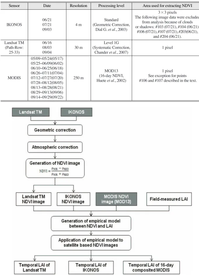
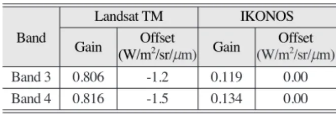
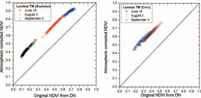
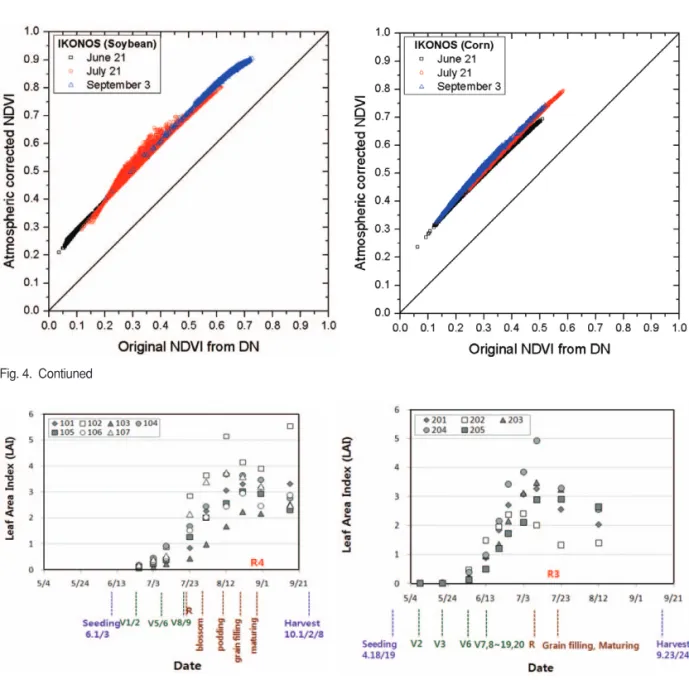
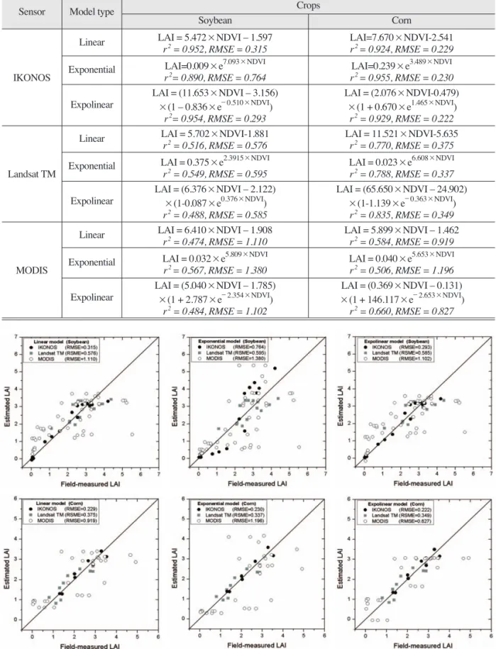
Abstract : Leaf area index (LAI) is important in explaining the ability of the crop to intercept solar energy for biomass production and in understanding the impact of crop management practices. This paper describes a procedure for estimating LAI as a function of image-derived vegetation indices from temporal series of IKONOS, Landsat TM, and MODIS satellite images using empirical models and demonstrates its use with data collected at Missouri field sites. LAI data were obtained several times during the 2002 growing season at monitoring sites established in two central Missouri experimental fields, one planted to soybean (Glycine max L.) and the other planted to corn (Zea mays L.). Satellite images at varying spatial and spectral resolutions were acquired and the data were extracted to calculate normalized difference vegetation index (NDVI) after geometric and atmospheric correction.

Linear, exponential, and expolinear models were developed to relate temporal NDVI to measured LAI data. Models using IKONOS NDVI estimated LAI of both soybean and corn better than those using Landsat TM or MODIS NDVI.

Expolinear models provided more accurate results than linear or exponential models.

Key Words : leaf area index, NDVI, IKONOS, Landsat TM, MODIS, Missouri

Received October 18, 2012; Revised November 5, 2012; Accepted November 7, 2012.

†

Corresponding Author: Suk Young Hong([email protected])

This is an Open-Access article distributed under the terms of the Creative Commons Attribution Non-Commercial License

(http://creativecommons.org/licenses/by-nc/3.0) which permits unrestricted non-commercial use, distribution, and reproduction in

any medium, provided the original work is properly cited.

normalize internal effects such as canopy background variations. In spectral signature analysis by remote sensing, vegetation indices that combine red and near-infrared bands are widely used for estimating the vitality and the productivity of vegetation. The cellular structure of leaf mesophyll strongly scatters and reflects near-infrared energy. In the visible region, vegetation looks dark on the imagery because of the high absorption of pigments such as chlorophylls(Jensen, 2000). Although these physical bases explain their function, vegetation indices are generally based on empirical evidence, not on basic biology, chemistry or physics.

Remote sensing estimation of LAI has been primarily based on the empirical relationship between the field-measured LAI and satellite image-based spectral signals (Curran et al., 1992; Peddle et al., 1999). As a single value to represent the remotely sensed spectral responses of vegetation, spectral vegetation indices, such as the normalized difference vegetation index (NDVI) as shown in Equation 1 or simple ratio, are frequently used to indirectly estimate LAI (Lee et al., 2006; Baret and Guyot, 1991; Huete et al., 1994; Potithep et al., 2010). Many previous studies investigated the relationship between LAI and NDVI, and developed empirical models based on that relationship (Turner et al., 1999; Gonzalez-Sanpedro et al., 2008; Zheng and Moskal, 2009; Kim and Lee, 2003). However, few studies compared LAI estimation based on data from various satellite sensors.

NDVI = (1)

r

: Reflectance of near-infrared band r

: Reflectance of red visible band

Many have attempted to develop relationships between LAI and vegetation indices for crop yield assessment and have discussed their potential and limitations (Baret and Guyot, 1991; Wiegand et al.,

1991; Thenkabail et al., 2000; Hong et al., 2004;

Doraiswamy et al., 2005). Jongschaap (2006) addressed LAI is often used for the crop growth model calibration leading to substantial improvement in the predictions. There is not a simple way to explain crop yield since it is influenced by many biotic and abiotic factors including weather condition and disease, Launay and Guerif (2005) reported spatial and temporal distribution of LAI estimates from remote sensing data was appealing to improve yield forecast. The objective of this study is to estimate LAI as a function of image-derived vegetation indices from temporal series of IKONOS, Landsat TM, and MODIS satellite data using empirical models and field data from Missouri field sites.

2. Materials and Methods

1) Study areas and monitoring sites

Data were collected on two fields (Field A, 36 ha and Field B, 13 ha) located within 3 km of each other near Centralia, in central Missouri (39.2 N, 92.1 W), USA as shown in Fig. 1. The soils found at these sites are classified as Aqualfs and are commonly referred to claypan soils. They are poorly drained and have a restrictive, high-clay layer (the claypan) occurring below the topsoil. Because of extensive weathering, the claypan soil is usually low in natural fertility and pH. Plant available water capacity is low because a large portion of the stored water is retained with the clay at the wilting point. Topsoil depth and landscape position influence water holding capacity and water flow within the fields, having a direct impact on crop yield (Kitchen et al., 1999).

The selection of within-field monitoring sites for this study was based on existing topography, topsoil depth, and historic yield information (Fraisse et al., r

_ r

r

+ r

Fig. 1. Locations of Field A and Field B in Centralia, Missouri, USA.

Fig. 2. Crop monitoring sites in the Field A for soybean and Field B for corn in 2002.

Field A

2001). The main goal was to select and properly place enough sites to adequately characterize the yield variability measured in the fields. Seven monitoring sites were selected in Field A (Sites 101- 107) and five were selected in Field B (Sites 201- 205) as shown in Fig. 2.

Data for this study were collected in 2002. Field A was planted to soybean on June 1 and June 3 (76 cm row spacing, 408,000 seeds/ha) and Field B was planted to corn on April 18 and April 19 (76 cm row spacing, 69,000 seeds/ha). Field A was managed with minimum tillage, while Field B was managed with no-tillage. Harvest was on October 1, 2, and 8 for Field A and September 23 and 24 for Field B.

Destructive crop sampling for LAI was carried out with a 1-m row section for corn and three 1-meter row sections for soybean. Corn measurements were obtained on 05/09, 05/21, 06/04, 06/13, 06/20, 06/25, 07/03, 07/10, 07/23, and 08/12, while soybean measurements were obtained on 06/20, 06/25, 07/03, 07/10, 07/23, 08/01, 08/12, 08/21, 08/31, and 09/16.

Leaf area was measured with a LI-COR1) leaf area meter (LI-3100), where the projected image of a leaf sample traveling under a fluorescent light source is reflected by a system of mirrors to a solid-state

scanning camera. Hatfield et al. (1976) reported that measurement error with this type of area meter is generally less than 2%. Growth stages for soybean and corn were also surveyed at each sampling date according to the handbook of ‘How a Soybean Plant Develops (Iowa State University, 1997a)’ and ‘How a Corn Plant Develops (Iowa State University, 1997b)’.

2) Image data used and image processing Multi-sensor optical data from IKONOS (4 m), Landsat TM (30 m), and MODIS (250 m) satellites were acquired for Field A and Field B on multiple dates from May to September during the 2002 cropping season (Table 1). Areas for extracting NDVI from the images were selected to be coincident with the hand-harvested areas for estimating LAI.

Field measurement data were interpolated using two adjacent dates to match the dates for images and paired with the image data value extracted from the one coincident pixel of the Landsat TM and MODIS images for data analysis. The one exception was for sites 106 and 107, which were located within the same MODIS image pixel. The LAI value corresponding to this pixel was determined by Fig. 2. Contiuned

Field B

Table 1. Multi-sensor optical image data acquired in 2002

Sensor Date Resolution Processing level Area used for extracting NDVI 3×3 pixels

06/21 Standard The following image data were excluded

IKONOS 07/21 4 m (Geometric Correction, from analysis because of clouds 09/03 Dial G. et al., 2003) or shadows: #103 (07/21), #104 (06/21),

#106 (07/21), #107 (07/21), #203(06/21), and #204 (06/21).

Landsat TM 06/16 Level 1G

(Path-Row: 08/03 30 m (Systematic Correction, 1 pixel

25-33) 09/04 Chander et al., 2007)

05/09~05/24(05/17) 05/25~06/09(06/02) 06/10~06/25(06/18)

MOD13 1 pixel

06/26~07/11(07/04)

(16-day NDVI, See exception for points MODIS 07/12~07/27(07/20) 250 m

Huete et al., 2002) #106 and #107 described in the text.

07/28~08/12(08/05) 08/13~08/28(08/21) 08/29~09/13(09/06) 09/14~09/29(09/22)

Sensor Date Resolution Processing level Area used for extracting NDVI

Fig. 3. Flow chart of the image processing and analysis procedures used in this study.

averaging the data values from two sites. Because IKONOS pixels were much smaller, the effect of different averaging windows (1 ×1, 3×3, and 5×5 pixels) was evaluated. Because IKONOS NDVI from the 3× 3 pixel window size had the highest correlation to LAI (data not shown), those data were used for further data analysis. Some IKONOS data were excluded from the analysis because of clouds or shadows as shown in Table 1.

Fig. 3 shows a flow chart of the image processing and analysis steps used in this study. Image data were first standardized for sensor comparison. The MODIS products (MOD13) used in this study were pre- processed atmospherically and geometrically by the image provider (Huete et al., 2002). Pre-processed MODIS images were reprojected from sinusoidal to UTM projection with zone 15 using the MODIS Reprojection Tool provided by the National Aeronautics and Space Administration (NASA, USA).

Atmospheric correction, which is a process to reduce atmospheric effects and more accurately estimate surface reflectance, was applied to the IKONOS and Landsat TM images using the COST model (Chavez, 1996). Based on Equation 2, Landsat TM and IKONOS digital numbers were converted to radiance values using radiometric calibration coefficients for each band as shown in Table 2.

Radiometric calibration coefficients for Landsat TM were obtained from the metadata file of the image.

Radiometric calibration coefficients developed by the NASA calibration team (Pagnutti et al., 2003) were

used for IKONOS images.

L

= gain

× DN

+ offset

(2) The COST model is an image-based atmospheric correction method. Radiance images calculated from Equation 2 are converted to reflectance images based on Equation 3. The COST model uses the cosine of the sun zenith angle for approximating the effects of absorption by the atmosphere. In Equation 4, path radiance due to haze (L

) can be calculated by subtracting L

from the at-satellite radiance of hazy objects as shown in Equation 5. The basic assumption is that dark objects comprise 1 percent minimum reflectance (Chavez, 1996). By correcting haze effects, the images are corrected band by band for atmospheric and radiometric noise (Chavez, 1996).

r

= (3)

where, L

= L

_ L

(4)

L

= (5)

r: spectral reflectance of the surface q: solar zenith angle

ESUN: top of the atmospheric solar irradiance d: distance between sun and earth

L

: at-sensor radiance for each band i

L

: path radiance due to haze for each band i L

: radiance of an absolutely dark object when it is

haze-free

L

: minimum radiance of each band i

Linear, exponential, and expolinear models (Anderson et al., 2004) as shown in Table 3 were used to estimate image-based LAI and compared with observed LAI. Although the linear model is simple to apply, performance of this model is poor during periods of Maximum LAI (Wang et al., 2005). For deciduous forest, the exponential model was more effective than the linear model (Tagesson, 2006). The expolinear model, which combined both linear and exponential functions, was used for modelling crop

0.01×ESUN

cosq

pd

pd

(L

_ L

)

ESUN

cosq

Table 2. Radiometric calibration coefficients for Landsat TM and IKONOS images

Landsat TM IKONOS

Band Gain Offset Gain Offset

(W/m

/sr/mm) (W/m

/sr/mm)

Band 3 0.806 -1.2 0.119 0.00

Band 4 0.816 -1.5 0.134 0.00

Landsat TM IKONOS

Band Gain Offset

Gain Offset

(W/m

/sr/mm) (W/m

/sr/mm)

growth and provided consistency between retrieved biophysical properties (Lee et al., 2003; Anderson et al., 2004). For the comparison of three models, coefficient of determination (r

) and root mean square error (RMSE) were used.

3. Results and Discussion

1) Atmospheric correction effect on IKONOS and Landsat TM images

NDVI values of IKONOS and Landsat TM atmospherically corrected using the COST model were compared with the NDVI values calculated from digital numbers of original images (Fig. 4). The relationship between NDVI values before and after atmospheric correction followed a strong linear

relationship as shown in Fig. 4, which reflects linear equation of COST model algorithm. NDVI values of IKONOS and Landsat TM after atmospheric correction were approximately 0.2 to 0.3 higher than those values from digital numbers of original images.

Minimum radiance (L

) of red band had generally higher values than that of near infrared band because of higher scattering in the visible band than in the near infrared band meanwhile radiance of an absolutely dark object when it is haze-free (L

) are the same in the red and near infrared bands. This resulted in higher spectral reflectance (r) of near infrared band and then higher NDVI values after atmospheric correction. Two sensor’s NDVIs using atmospheric corrected reflectance could be objectively compared as absolute value removed atmospheric effect. The range of IKONOS and

Fig. 4. Comparison of NDVI values before and after atmospheric correction of Landsat TM and IKONOS images in soybean and corn fields.

Table 3. Models used for estimating LAI from satellite NDVI values

Model Equations

Linear LAI = a×NDVI + b

Exponential LAI = a×exp

Expolinear LAI = (a×NDVI + b)×(1 + c×exp

)

Model Equations

Landsat TM NDVI values was wider in soybean than in corn. The NDVI range of IKONOS was larger than that of Landsat TM, which is because high spatial resolution of IKONOS image provides more detail spatial variability than Landsat TM does.

2) Crop growth and NDVI change

The LAI of soybean and corn at all monitoring sites increased to about 3~4 until the maturing stage(R4) at the end of August for soybean and until

the grain filling stage(R3) in mid-July for corn, and then decreased as shown in Fig. 5. Time difference for LAI peak for soybean and corn was about a month. Within-field LAI variability was found at both fields, with higher LAI variability among monitoring sites before the reproductive stages.

Soybean NDVI values calculated from IKONOS, Landsat TM, and MODIS at the sampling sites increased to about 0.9 until early September as shown in Fig. 6. Corn NDVI values increased to about 0.7 to Fig. 4. Contiuned

Fig. 5. LAI change of soybean (a) and corn (b) during the 2002 growing season.

Soybean in Field A Corn in Field B

0.8 in late July or early August and then decreased everywhere except site 202. Site 202 was located in a highly eroded sloped area. Low topsoil depth and low

water-holding capacity at this site, coupled with low precipitation in July and August (Jung et al., 2005), led to poor corn growth.

It was not easy to estimate the time of peak NDVI using IKONOS or Landsat TM data because only three images were obtained from each satellite during the 2002 crop growth season. Although timely acquisition of satellite imagery was known as one of limitations of remote sensing, IKONOS can be obtained more frequently because of shorter revisiting time. Landsat TM has a fixed temporal resolution as 16 days, which gives harder time to get time-series images during crop growing season. MODIS images are obtained each day but their coarse spatial resolution has a limitation to characterize field-level crop properties.

3) LAI estimation using NDVI values

Linear, exponential, and expolinear models were applied to estimate LAI using NDVI values from IKONOS, Landsat TM, and MODIS images as shown in Table 4. Expolinear models showed higher r2 than linear and exponential models for corn LAI estimation. Anderson et al. (2004) indicated “One functional advantage to the expolinear regression form is that the linear section (at low VI) extrapolates to bare soil conditions at reasonable values of VI ” . For soybean, expolinear model showed the highest r2 value from IKONOS-derived models for LAI estimation but linear and exponential models showed the highest r

value from Landsat TM- and MODIS- derived models, respectively.

All IKONOS-derived models for LAI estimation had higher r2 values than Landsat TM- or MODIS- derived models, which implied satellite images with higher spatial resolution were more useful for estimating within-field LAI variability than those with coarser spatial resolution such as Landsat TM and MODIS(Table 4).

Fig. 6. NDVI calculated from IKONOS (a), Landsat TM (b), and MODIS (c) images at soybean (#101~#107) and corn (#201~#205) monitoring sites during growing period in 2002.

(c)

(b)

(a)

Fig. 7. Comparison between measured and estimated LAI with linear, exponential, and expolinear equations from satellite NDVI values for soybean (top) and corn (bottom).

Table 4. LAI prediction models using IKONOS, Landsat TM, and MODIS NDVI values for soybean and corn

Sensor Model type Crops

Soybean Corn

Linear LAI = 5.472×NDVI _ 1.597 LAI=7.670×NDVI-2.541

r

= 0.952, RMSE = 0.315 r

= 0.924, RMSE = 0.229

Exponential LAI=0.009×e

LAI=0.239×e

IKONOS r

= 0.890, RMSE = 0.764 r

= 0.955, RMSE = 0.230

LAI = (11.653×NDVI _ 3.156) LAI = (2.076×NDVI-0.479) Expolinear ×(1 _ 0.836×e

) ×(1 + 0.670×e

)

r

= 0.954, RMSE = 0.293 r

= 0.929, RMSE = 0.222

Linear LAI = 5.702×NDVI-1.881 LAI = 11.521×NDVI-5.635

r

= 0.516, RMSE = 0.576 r

= 0.770, RMSE = 0.375 Exponential LAI = 0.375×e

LAI = 0.023×e

Landsat TM r

= 0.549, RMSE = 0.595 r

= 0.788, RMSE = 0.337

LAI = (6.376×NDVI _ 2.122) LAI = (65.650×NDVI _ 24.902) Expolinear ×(1-0.087×e

) ×(1-1.139×e

) r

= 0.488, RMSE = 0.585 r

= 0.835, RMSE = 0.349

Linear LAI = 6.410×NDVI _ 1.908 LAI = 5.899×NDVI _ 1.462

r

= 0.474, RMSE = 1.110 r

= 0.584, RMSE = 0.919 Exponential LAI = 0.032×e

LAI = 0.040×e

MODIS r

= 0.567, RMSE = 1.380 r

= 0.506, RMSE = 1.196

LAI = (5.040×NDVI _ 1.785) LAI = (0.369×NDVI _ 0.131) Expolinear ×(1 + 2.787×e

) ×(1 + 146.117×e

) r

= 0.484, RMSE = 1.102 r

= 0.660, RMSE = 0.827

Sensor Model type Crops

Soybean Corn

Differences between IKONOS-derived LAI and measured LAI were lower than for Landsat TM- derived or MODIS-derived LAI for both soybean and corn (Fig. 7). The expolinear models generally provided better results, as shown both by higher r2 values and lower RMSE than linear or exponential models. The RMSE for corn LAI estimation, in general, was lower than for soybean LAI estimation (Table 4).

The reason that NDVI-based expolinear model performed better for LAI estimation than linear or exponential models can be explained that expolinear model is closer to crop growth pattern, which combines linear and exponential curves at the same time during the growing period (Anderson et al., 2004; Lee et al., 2003). Although recent studies used time-series MODIS NDVI data to monitor crop LAI and growth (Breuning et al., 2011; Wardlow et al., 2007), NDVI from satellite images with higher spatial resolution such as IKONOS were more useful for estimating within-field LAI or crop growth variability than those with coarser spatial resolution including Landsat TM and MODIS in this study

4. Conclusions

LAI is important in explaining the ability of the crop to intercept solar energy for biomass production and in understanding the impact of crop management practices. For improved efficiency of measurement, soybean and corn LAI was estimated using IKONOS, Landsat TM, and MODIS NDVI values. After geometric and atmospheric correction, field- measured LAI was modelled as a function of NDVI using linear, exponential, and expolinear regression models. Soybean NDVI values calculated from IKONOS, Landsat TM, and MODIS increased to about 0.9 until early September and corn NDVI

values increased to about 0.7~0.8 until late July or early August. The IKONOS-derived models for provided higher r2 values than Landsat TM- or MODIS-derived models, which implied satellite images with higher spatial resolution were more useful for estimating within-field LAI variability than those with coarser spatial resolution. Based on RMSE, the expolinear model generally fit the data better than linear or exponential models for both soybean and corn. We suggest remote sensing estimates of LAI from satellite images with high spatial resolution can provide estimates of spatial variability in LAI, which is of use in modelling of crop growth and yield.

Acknowledgement

This study was supported by 2012 Post-doctoral Fellowship Program (Project No. PJ007753022012) of National Academy of Agricultural Science, Rural Development Administration, Republic of Korea.

References

Anderson, M.C., C.M.U. Neale, F. Li, J.M. Norman, W.P. Kustas, H. Jayanthi, and J. Chavez, 2004. Upscaling ground observations of vegetation water content, canopy height, and leaf area index during SMEX02 using aircraft and Landsat imagery, Remote Sensing of Environment, 92: 447-464.

Baret, F. and G. Guyot, 1991. Potentials and limits of vegetation indices for LAI and aFAR assessment, Remote Sensing of Environment, 35: 161-173.

Breunig, F.M., L.S. Galvao, A.R. Formaggio, and

J.C.N. Epiphanio, 2011. Directional effects

on NDVI and LAI retrievals from MODIS:

A case study in Brazil with soybean, International Journal of Applied Earth Observation and Geoinformation, 13: 34-42.

Chander, G., B.L. Markham, and J.A. Barsi, 2007.

Revised Landsat-5 Thematic Mapper radiometric calibration, IEEE Geoscience and Remote Sensing Letters, 4(3): 490-494.

Cohen, W.B., T.K. Maiersperger, Z. Yang, S.T.

Gower, D.P. Turner, W.D. Ritts, M.

Berterretche, and S.W. Running, 2003.

Comparisons of land cover and LAI estimates derived from ETM+ and MODIS for four sites in North America: a quality assessment of 2000/2001 provisional MODIS products, Remote Sensing of Environment, 88: 233-255.

Curran, P.J., J. Dungan, and H.L. Gholz, 1992.

Seasonal LAI measurements in slash pine using Landsat TM, Remote Sensing of Environment, 39: 3-13.

Dial, G., H. Bowen, F. Gerlach, J. Grodecki, and R.

Oleszczuk, 2003. IKONOS satellite, imagery, and products, Remote Sensing of Environment, 88: 23-36.

Doraiswamy, P.C., T.R. Sinclair, S. Hollinger, B.

Akhmedov, A. Stern, and J. Prueger, 2005.

Application of MODIS derived parameters for regional crop yield assessment, Remote Sensing of Environment, 97: 192-202.

Fraisse, C.W., K.A. Sudduth, N.R. Kitchen, 2001.

Calibration of the ceres-maize model for simulating site-specific crop development and yield on claypan soils, Applied Engineering in Agriculture. 17(4): 547-556.

Gonzalez-Sanpedro, M.C., T.L. Toan, J. Moreno, L.

Kergoat, and E. Rubio, 2008. Seasonal variations of leaf area index of agricultural fields retrieved from Landsat data, Remote Sensing of Environment, 112: 810-824.

Hatfield, J.L., C.D. Stanley, and R.E. Carlson, 1976.

Evaluation of an electronic foliometer to measure leaf area in corn and soybean, Agronomy Journal, 68: 434-436.

Hong, S.Y., K.A. Sudduth, N.R. Kitchen, C.W.

Fraisse, H.L. Palm, and W.J. Wiebold, 2004.

Comparison of remote sensing and crop growth models for estimating within-field LAI variability, Korean Journal of Remote Sensing, 20(3): 175-188.

Huete, A., C. Justice, and H. Liu, 1994. Development of vegetation and soil indices for MODIS- EOS, Remote Sensing of Environment, 49:

224-234.

Huete, A., K. Didan, T. Miura, E.P. Rodriguez, X.

Gao, and L.G. Ferreira, 2002. Overview of the radiometric and biophysical performance of the MODIS vegetation indices, Remote Sensing of Environment, 83: 195-213.

Iowa State University of Science and Technology Cooperative Extension Service, 1997a. How a corn plant develops, Special Report No. 48.

Iowa State University of Science and Technology Cooperative Extension Service, 1997b. How a soybean plant develops, Special Report No.

53.

Jensen, J.R., 2000. Remote sensing of the environment;

An earth resource perspective, Prentice Hall, p.197

Jongschaap, R.E.E., 2006. Run-time calibration of simulation models by integrating remote sensing estimates of leaf area index and canopy nitrogen, European Journal of Agronomy, 24: 328-336.

Kim, S.H. and K.S. Lee, 2003. Local validation of MODIS global Leaf Area Index (LAI) product over temperate forest, Korean Journal of Remote Sensing, 19(1): 1-9.

Kitchen, N.R., Sudduth, K.A., and Drummond, S.T.,

1999. Soil electrical conductivity as a crop productivity measure for claypan soils, Journal of Production Agriculture, 12: 607- 617.

Launay, M. and M. Guerif, 2005. Assimilating remote sensing data into a crop model to improve predictive performance for spatial applications, Agriculture, Ecosystems &

Environment, 111: 321-339.

Lee, J.H., J. Goudriaan, and H. Challa, 2003. Using the expolinear growth equation for modelling crop growth in year-round cut chrysanthemum, Annals of Botany, 92: 697-708.

Lee, K.S., S.H. Kim, J.H. Park, T.G. Kim, Y.I. Park, and C.S. Woo, 2006. Estimation of forest LAI in close canopy situation using optical remote sensing data, Korean Journal of Remote Sensing, 22(5): 305-311.

Mahiny, A.S. and B.J. Turner, 2007. A comparison of four common atmospheric correction methods, Photogrammetric Engineering and Remote Sensing, 73(4): 361-368.

Pagnutti, M., R.E. Ryan, M. Kelly, K. Holekamp, V.

Zanoni, K. Thome, and S. Schiller, 2003.

Radiometric characterization of IKONOS multispectral imagery, Remote Sensing of Environment, 88: 53-68.

Peddle, D.R., F.R. Hall, and E.F. LeDrew, 1999.

Spectral mixture analysis and geometricoptical reflectance modeling of boreal forest biophysical structure, Remote Sensing of Environment, 67: 288-297.

Potithep, S., N.K. Nasahara, H. Muraoka, S.

Nagai, R. Suzuki, 2010. What is the actual relationship between LAI and VI in a deciduous broadleaf forest?, International Archives of the Photogrammetry, Remote Sensing and Spatial Information Science, 11152(8): 609-614.

Tagesson, T., 2006. Indirect estimations and spatial variation in Leaf Area Index of coniferous, deciduous and mixed forest stands in Forsmark and Laxemar, SKB TR-06-29 (Stockholm:Swedish Nuclear Fuel and Waste Management Co.).

Thenkabail, P.S., R.B. Smith, and E. De Pauw, 2000.

Hyperspectral vegetation indices for determining agricultural crop characteristics, Remote Sensing of Environment, 71: 158-182.

Turner, D., W. Cohen, R. Kennedy, K. Fassnacht, and J. Briggs, 1999. Relationships between leaf area index and Landsat TM spectral vegetation indices across three temperature zone sites, Remote Sensing of Environment, 70: 52-68.

Wang, Q., S. Adiku, J. Tenhunen, and A. Granier, 2005. On the relationship of NDVI with leaf area index in a deciduous forest site, Remote Sensing of Environment, 94: 244-255.

Wardlow, B.D., S.L. Egbert, and J.H. Kastens, 2007.

Analysis of time-series MODIS 250 m vegetation index data for crop classification in the U.S. Central Great Plains, Remote Sensing of Environment, 108: 290-310.

Watson, D.J., 1947. Comparative physiological studies on the growth of field crops: I.

Variation in net assimilation rate and leaf area between species and varieties, and with and between years. Annual. Botany, (N.S.), 11:

41-76.

Wiegand, C.L., A.J. Richardson, D.E. Escobar, and A.H. Gerbermann, 1991. Vegetation indices in crop assessments, Remote Sensing of Environment, 35: 105-119.

Zheng, G. and L.M. Moskal, 2009. Retrieving leaf area index (LAI) using remote sensing:

Theories, methods and sensors, Sensors, 9:

2719-2745.