Tests for the exponential distribution based on Type-II censored samples

Tests for the exponential distribution based on Type-II censored samples

Suk-Bok Kang ¹⁾ ․ Young-Suk Cho ²⁾ ․ Sei-Yeon Choi ³⁾

Abstract

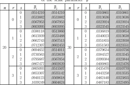
Two explicit estimators of the scale parameter in an exponential distribution based on Type-II censored samples are proposed by appropriately approximating the likelihood function. Then two type tests, including the modified Cramer-von Mises test and Kolmogorov-Smirnov test are developed for the exponential distribution based on Type-II censored samples by using the proposed estimators.

For each test, Monte Carlo techniques are used to generate critical values. The powers of these tests are investigated under several alternative distributions.

Keywords : Exponential distribution, Type-II censored samples, Cramer-von Mises test, Kolmogorov-Smirnov test

1. Introduction

Consider an exponential distribution with the probability density function (pdf) f( x ;θ) = 1

θ e

, x ＞0, θ ＞0 (1.1)

and the cumulative distribution function (cdf)

1) Professor, Department of Statistics, Yeungnam University, 214-1, Daedong, Kyongsan, Kyoungbuk, 712-749, Korea

E-mail: [email protected]

2) Full-time Lecturer, Department of Applied Economics, Miryang National University 1025-1, Naeidong, Miryang, Kyoungnam, 627-130, Korea

3) Department of Statistics, Yeungnam University, 214-1, Daedong, Kyongsan, Kyoungbuk,

712-749, Korea

F( x ;θ) = 1 - e

, x ＞0 , θ ＞0 (1.2) The exponential distribution has been used as models in analyzing life-time data quite extensively. Kambo (1978) proposed the maximum likelihood estimators of the location and scale parameters of the exponential distribution from a censored sample. Balakrishnan (1990) studied the maximum likelihood estimation of the parameters in the exponential distribution based on multiplying Type-II censored sample. Balasubramanian and Balakrishnan (1992) proposed the approximate maximum likelihood estimation of parameters based on censored samples under one-parameter and two-parameter exponential distributions.

The Cramer-von Mises goodness-of-fit test statistics is given by W _n

= n ⌠ ⌡

∞

- ∞

[F _n (x) - F

(x)]

dF

(x) (1.3) where _{F n (x)} is the empirical distribution function of _X

_{, ..., X n} and _F

_(x) is the cumulative distribution functions assumed under _H

. But _{W n}

of (1.3) can only be used with complete samples.

Sirvanci and Levent (1982) employed the modified form of the Cramer-von Mises statistic for the problem of testing exponentiality with Type-I censored samples and they obtained the asymptotic distribution of the Cramer-von Mises statistic. Porter Ⅲ, Coleman, and Moore (1992) developed three modified empirical distribution function type tests, the Kolmogorov-Smirnov (K-S), Anderson-Darling (A-D), Cramer-von Mises (C-vM), for the Pareto distribution with unknown parameters of location and scale and known shape parameter based on complete samples.

Let _X

_{, ...,X n} be a random sample from the exponential distribution with pdf (1.1), and let _X

_≤X

_{≤…≤X n :n} be the corresponding order statistics.

In this paper, two tests of the modified K-S and C-vM are developed for the one-parameter exponential distribution based on Type-II censored samples. The unknown parameter is estimated by using two approximate maximum likelihood estimation methods. For each test, we generate critical values for sample sizes n = 20, 30 and various choices of censoring. We also compare the powers of these modified tests under several alternative distributions.

2. Estimations of the scale parameter

Assume that

X r + 1 : n ≤ X r + 2 : n ≤…≤X n - s : n (2.1) is the available Type-II censored sample from the exponential distribution with pdf (1.1), where the first _r and the last _s observations are censored.

The likelihood function based on the Type-II censored sample in (2.1) is given by

L = n!

r!s! { F( X r + 1 : n ; θ)} ^r {1 - F( X n - s : n ; θ)} ^s ∏

n - s

i = r + 1 f(X i : n ; θ) (2.2)

By putting _{Z i : n = X i : n /θ} , L = n!

r!s! θ

{ F( Z r + 1 : n )} ^r {1 - F( Z n - s : n )} ^s ∏

n - s

i = r + 1 f(Z i : n ) (2.3)

where A = n - r - s is the size of the censored sample, _{f(z) = e}

and F(z) = 1 - e

are the pdf and cdf of a standard exponential distribution, respectively. Then the log-likelihood function is given by

ln L = ln ( r!s! ^n! ) - A ln θ + r ln { F( Z r + 1 : n )}

+ s ln { 1 - F( Z _{n - s : n} )} + ∑ ^{n - s}

i = r + 1 lnf( Z _{i : n} ).

(2.4)

On differentiating with respect to _θ in turn and equation to zero, we obtain an estimating equation as

∂ ln L

∂θ = - 1

θ [ ^{A + r f( Z F(Z r + 1 : n r + 1 : n )Z r + 1 : n ) - s 1 - F( Z f( Z n - s : n n - s : n ) ) Z n - s:n}

+ ^{n - s} ∑

i = r + 1

f ' ( Z i : n )

f( Z i : n ) Z i : n ] ^{= 0.}

(2.5)

Since the likelihood equation is very complicated, the equation (2.5) does not admit explicit solution for _θ . But we may expand the functions ^{f( Z r + 1:n )}

F( Z r + 1:n ) and f( Z _{r + 1 : n} )Z _{r + 1 : n}

F(Z _{r + 1 : n} ) in Taylor series around the point _{a ≡ F}

_{(p r + 1} ) = - ln (q _{r + 1} ) , where _{p i =} ⁱ

n + 1 and _{q i = 1 - p i} .

Therefore, we may approximate these functions by Taylor expansion as f(Z r + 1:n )

F( Z r + 1:n ) ≃α

- β

Z r + 1:n (2.6)

f(Z r + 1:n )Z r + 1 : n

F(Z _{r + 1:n} ) ≃ α

+ β

Z _{r + 1:n} (2.7)

where

α

= n - r

r + 1 + ( n + 1)( n - r )

( r + 1)

ln ( ^{n - r} n + 1 ) ^{, β}

⁼ ( n + 1)( n - r ) ( r + 1)

, α

= q r + 1 ( ln q r + 1 )

p

r + 1

, _β

₌ ^{q r + 1 ( p r + 1 + ln q r + 1 )} p

r + 1

.

From equations (2.6) and (2.7), the approximate likelihood equations for _θ are given by

∂ ln L

∂θ ≃ ∂ ln L

∂θ = - 1

θ [ A + rZ r + 1:n (α

- β

Z r + 1:n )

- sZ _{n - s:n} - ∑

n - s

i = r + 1 Z _i:n ] ^{= 0}

(2.8)

and

∂ ln L

∂θ ≃ ∂ ln L

∂θ = - 1

θ [ A + rZ r + 1:n (α

- β

Z r + 1:n ) - sZ n - s:n - ∑ ^{n - s}

i = r + 1 Z i:n ] ^{= 0}

(2.9)

On solving equation (2.8) for θ, we can derive an approximate maximum likelihood estimator (AMLE) of θ as

θ

= - B

+ B

- 4AC

2A (2.10)

where

_B

₌ ( ^r ( ^{n - r r + 1 +} ( n + 1)( n - r )

( r + 1)

ln ( ^{n - r} n + 1 ) ) ^{X r + 1 : n - sX n - s : n - i = r + 1 ∑ n - s X i : n} ) ^,

_C

_{= - r} ( n + 1)( n - r )

( r + 1)

X

r + 1 : n .

From equation (2.9), we can derive more simple estimator which is a linear function of the order statistics than _θ

as follows;

θ

=

- r β

X _{r + 1 : n} + s X _{n - s : n} + ∑

n - s i = r + 1 X _{i : n} A+rα

(2.11)

From the equations (2.10) and (2.11), the mean squared errors (MSE) of these

two estimators are simulated by Monte Carlo method for sample sizes n = 20( 30)

and various choices of censoring. These values are given in Table 1. From Table

1, we can obtain the following results; _θ

is generally more efficient and simple

than _θ

in the sense of MSE. So _θ

is not only very simple estimator but also

better estimator than _θ

in the sense of the MSE. Obviously, when _{r = 0} , two

estimators are same.

3. Goodness-of-fit tests

Porter Ⅲ et. al. (1992) developed the modified empirical distribution function type tests that are the K-S test and C-vM test for complete samples. An estimator was used to find the hypothesized cdf: _{P i = F( x i :n , θ )} , i = 1 , ..., n . Then the values of the two modified test statistics were calculated as follows;

The K-S test statistic was computed:

D = max { D

,D

} , (3.1)

D

≡ sup

| [ ( n ⁱ ) ^{- P i} ]| ^{, (3.2)}

D

≡ sup

| [ ^{P i -} ( n ⁱ )]| ^{. (3.3)}

The C-vM test statistic was computed:

. (3.4)

But these tests can not use for the censored samples. One of the assumptions frequently employed in life testing is that the items, which are put on test, have an exponential distribution. The data for estimating the parameter _θ is usually obtained through a censored sampling scheme. So, we propose the modified K-S test and C-vM test by using the proposed AMLEs _θ

_{and θ}

based on Type-II censored samples. For _{k = 1, 2} , two test statistics are developed as follows;

The modified K-S test statistic:

D k = max { ^D

^{k ,D}

^k } ^{, (3.5)}

D

k ≡ sup r + 1 ≤i≤ n - s | [ ( n - r - s ⁱ ) ^{- P i, k} ]| ^{, (3.6)}

D

_k ≡ sup r + 1 ≤i≤ n - s | [ ^{P i, k -} ( n - r - s ⁱ )]| ^{. (3.7)}

The modified C-vM test statistic:

(3.8) where _{P i, k = F( x i:n , θ k )} , i = r + 1, r + 2,..., n - s, k = 1 , 2 , _{F( x ;θ)} is the hypothe- sized cdf, and _{θ k} are AMLEs of _θ .

This procedure was repeated 10,000 times for each sample size n , two tests,

and _{k = 1, 2} . The 10,000 test statistics were then ordered for each of the two tests and _{k = 1, 2} . Then the 95th percentiles are found from these values. Critical values are contained in Table 2.

A power comparison was made between the modified C-vM and K-S goodness-of-fit tests for the one-parameter exponential distribution. The power values were determined by generating 10,000 random samples of size n = 20 for each of several distributions. Table 3 contains the powers for several alternative distributions.

From Table 3, we have the following results;

When the alternative distribution is beta and Weibull distributions, the modified K-S statistic _D

is generally more powerful test than the other tests. But when r = 0, s = 0( 1) and r = 1, s = 0 , the modified C-vM statistic _W

is generally more powerful test than the other tests. When the alternative distribution is gamma distribution, the modified K-S statistic _D

is also generally more powerful test than the other tests except r = 0 and s = 0 . When the alternative distribution is lognormal distributions and s is large, the modified K-S statistic D

is generally more powerful test than the other tests, but when s is small, the modified C-vM statistic _W

is generally more powerful test than the other tests.

Almost all cases, the tests based on the estimator _θ

are more powerful than the tests based on the estimator _θ

Table 1. The relative mean squared errors for the estimators of the scale parameter _θ

n r s θ

θ

n r s θ

θ

20 0

0 .0514210 .0514210

30 0

0 .0310861 .0310861

1 .0533882 .0533882 1 .0313636 .0313636

2 .0567953 .0567953 2 .0323924 .0323924

3 .0603095 .0603095 3 .0323545 .0323545

1

0 .0590118 0513860

1

0 .0336819 .0310854

1 .0615939 .0533488 1 .0340023 .0313638

2 .0662743 .0567513 2 .0351855 .0323938

3 .0712307 .0602453 3 .0351583 .0323551

2

0 .0694652 .0514011

2

0 .0379634 .0310756

1 .0730563 .0533639 1 .0384527 .0313545

2 .0795687 .0567854 2 .0399384 .0323844

3 .0867477 .0602620 3 .0400865 .0323476

3

0 .0805093 .0515507

3

0 .0435470 .0310770

1 .0853307 .0535142 1 .0443258 .0313535

2 .0940123 .0569618 2 .0462440 .0323855

3 .1039249 .0604624 3 .0467183 .0323495

Table 2. Critical values for the modified C-vM and K-S tests. ( _{α = 0.05} )

n r s W

D

W

D

20 0

0 .2173747 .2336347 .2173747 .2336347 1 .2332642 .2303864 .2332642 .2303864 2 .2795554 .2261714 .2795554 .2261714 3 .3543372 .2224418 .3543372 .2224418

1

0 .3322357 .2398282 .2441147 .2329285 1 .4567901 .2380075 .3068223 .2296714 2 .6005613 .2358128 .3959173 .2254914 3 .7662002 .2327945 .5151561 .2211034

2

0 .6234684 .2660206 .3322346 .2317841 1 .8382189 .2650682 .4451366 .2284472 2 1.0583520 .2646906 .5858888 .2242792 3 1.3026620 .2635810 .7526892 .2195999

3

0 1.0510270 .2902315 .5005844 .2295684 1 1.3621580 .2919133 .6660939 .2264541 2 1.6825810 .2913714 .8681232 .2215729 3 2.0078110 .2916449 1.0939050 .2171154

30 0

0 .2177687 .1931833 .2177687 .1931833 1 .2279940 .1911092 .2279940 .1911092 2 .2604270 .1898848 .2604271 .1898848 3 .3159882 .1868236 .3159883 .1868236

1

0 .2979723 .1961378 .2331697 .1927560 1 .3873298 .1954901 .2755975 .1907240 2 .4906859 .1943437 .3423309 .1894669 3 .6175565 .1932334 .4243127 .1865585

2

0 .5154319 .2142743 .2882550 .1923061 1 .6622366 .2145040 .3672278 .1906910 2 .8268008 .2150103 .4651260 .1891085 3 1.0022270 .2142496 .5747640 .1859771

3

0 .8084869 .2322742 .3878360 .1919480

1 1.0167880 .2327982 .4998192 .1899812

2 1.2377390 .2331694 .6297231 .1886678

3 1.4667920 .2338629 .7732853 .1857277

Table 3. Powers for several alternative distributions

n r s

Beta distribution with parameters 3 and 2 Beta(3, 2)

W

D

W

D

20 0

0 1.0000 .9989 1.0000 .9989

1 1.0000 .9973 1.0000 .9973

2 .9946 .9956 .9946 .9956

3 .9577 .9915 .9577 .9915

1

0 .9978 .9983 1.0000 .9991

1 .9410 .9956 .9962 .9974

2 .6102 .9904 .9645 .9954

3 .1196 .9830 .8023 .9905

2

0 .7513 .9872 .9979 .9988 1 .1142 .9728 .9637 .9971

2 .0003 .9445 .7825 .9939

3 .0000 .9008 .3307 .9885

3

0 .0017 .9387 .9634 .9983

1 .0000 .8724 .7487 .9961

2 .0000 .7823 .2461 .9923

3 .0000 .6460 .0086 .9842

n r s

Beta distribution with parameters 2 and 3 Beta(2, 3)

W

D

W

D

20 0

0 .9428 .8464 .9428 .8464

1 .8304 .7990 .8304 .7990

2 .6382 .7548 .6382 .7548

3 .3922 .7069 .3922 .7069

1

0 .6680 .8085 .8665 .8423

1 .2723 .7397 .6547 .7929

2 .0505 .6744 .4010 .7469

3 .0025 .6119 .1611 .6968

2

0 .0614 .6075 .6648 .8308

1 .0011 .5130 .3703 .7777

2 .0000 .4215 .1305 .7269

3 .0000 .3371 .0199 .6772

3

0 .0000 .3658 .3182 .8090

1 .0000 .2524 .0942 .7504

2 .0000 .1724 .0100 .6989

3 .0000 .1078 .0002 .6373

Table 3. (continued)

n r s

Gamma distribution with parameters 2 and 3 Gamma(2, 3)

W

D

W

D

20 0

0 .4912 .4149 .4912 .4149

1 .3602 .3924 .3602 .3924

2 .2336 .3784 .2336 .3784

3 .1227 .3622 .1227 .3622

1 0 .1564 .3577 .3409 .4036

1 .0364 .3303 .2066 .3838

2 .0046 .3009 .1008 .3693

3 .0007 .2747 .0319 .3532

2 0 .0028 .1742 .1614 .3760

1 .0002 .1484 .0656 .3546

2 .0000 .1183 .0204 .3379

3 .0000 .0945 .0039 .3238

3 0 .0000 .0604 .0367 .3412

1 .0000 .0402 .0099 .3160

2 .0000 .0291 .0020 .3006

3 .0000 .0204 .0008 .2840

n r s Weibull distribution with parameters 2 and 3 Weibull(2, 3) W

D

W

D

20 0 0 .9371 .8568 .9371 .8568

1 .8461 .8238 .8461 .8238

2 .6874 .7899 .6874 .7899

3 .4537 .7542 .4537 .7542

1 0 .6653 .8174 .8631 .8515

1 .2728 .7691 .6824 .8155

2 .0549 .7194 .4382 .7804

3 .0040 .6658 .1829 .7448

2 0 .0532 .6220 .6564 .8337

1 .0010 .5403 .3747 .7963

2 .0000 .4509 .1407 .7569

3 .0000 .3658 .0224 .7179

3 0 .0000 .3570 .2834 .8106

1 .0000 .2552 .0933 .7605

2 .0000 .1859 .0109 .7210

3 .0000 .1172 .0001 .6731

Table 3. (continued)

n r s

Lognormal distribution with parameters 0 and 1 LN(0, 1)

W

D

W

D

20 0

0 .1509 .1398 .1509 .1398

1 .1340 .1126 .1340 .1126

2 .1088 .1083 .1088 .1083

3 .0790 .1135 .0790 .1135

1 0 .0848 .1151 .1751 .1352

1 .0337 .0836 .1271 .1062

2 .0146 .0734 .0911 .1006

3 .0062 .0693 .0642 .1046

2 0 .0401 .0566 .1794 .1268

1 .0115 .0315 .1226 .0969

2 .0034 .0218 .0817 .0905

3 .0012 .0182 .0600 .0922

3 0 .0225 .0305 .1834 .1223

1 .0041 .0102 .1231 .0857

2 .0009 .0049 .0800 .0800

3 .0004 .0029 .0602 .0769

References

1. Balakrishnan, N. (1990). On the maximum likelihood estimation of the location and scale parameters of exponential distribution based on multiply Type-II censored samples, Journal of Applied Statistics, 17, 55-61.

2. Balasubramanian, K. and Balakrishnan, N. (1992). Estimation for one-parameter and two-parameter exponential distributions under multiple type-II censoring, Statistische Hefte, 33, 203-216.

3. Kambo, N. S. (1978). Maximum likelihood estimators of the location and scale parameters of exponential distribution from a censored sample, Commun. Statist,-Theor. Meth. A1(12), 1129-1132.

4. Porter III, J. E. and Coleman, J. W. and Moore, A. H. (1992). Modified KS, AD, and C-vM Tests for the Pareto Distribution with Unknown Location & Scale Parameters, IEEE Transactions on Reliability, 41(1), 112-117.

5. Sirvanci, M. and Levent, I. (1982). Cramer-von Mises statistic for testing exponentiality with censored samples, Biometrika, 69(3), 641-646.

[ received date : Jan. 2003, accepted date : May. 2003 ]