온대북부형 낙엽활엽수림의 디지털 카메라 반복 이미지를 활용한 식물계절 분석
한상학 1⋅윤충원 2⋅이상훈 1*
1국립생태원 기후변화연구팀, 2공주대학교 산림자원학과
Phenophase Extraction from Repeat Digital Photography in the Northern Temperate Type Deciduous Broadleaf Forest
Sang Hak Han
1, Chung Weon Yun
2and Sanghun Lee
1*1Team of Climate Change Research, National Institute of Ecology, Seocheon 33657, Korea
2Depatment of Forest Resources, Kongju National University, Yesan 32439, Korea
요 약: 매년 반복되는 식물의 생활사를 장기적으로 관측하는 것은 기후변화 반응을 감지하는데 있어 가장 단순한 방법이 며, 중요한 지표로 인식되고 있다. 반복 디지털 이미지를 이용한 식물계절 변화 관찰 방법은 전통적(현장에서 전문가에 의 해 관찰) 방법과 위성원격탐사(위성영상의 식생지수를 활용한 위성원격 관찰)의 한계를 보완한 방법이다. 본 연구는 디지 털 카메라를 기반으로 한 반복 이미지로부터 식물계절 변화 관측과 계절현상을 정량화하기 위하여 점봉산 산림생태계를 대상으로 하였다. 한반도 전역에 분포하는 신갈나무림(낙엽활엽수림)과 상록침엽수림의 대표 수종인 소나무를 선정하여 식 물계절 특성에 따른 경향성을 파악하고자 하였다. RGB 채널 이미지 데이터로부터 식생지수(Gcc)를 산출하였다. Gcc 진폭 의 크기는 상록침엽수림이 낙엽활엽수림 보다 작았으며, Gcc의 기울기(봄철 증가와 가을철 감소)는 상록침엽수림이 낙엽 활엽수림과 비교하여 완만하였다. 소나무림은 생장의 시작(UD)이 신갈나무림에 보다 빨랐고, 생장의 종료(RD)는 늦은 것 으로 나타났다. 식물계절 현상의 정확도 검증은 RMSE가 0.008(ROI1)과 0.006(ROI3)으로 높은 정확도를 보였다. 이러한 결과는 온대북부형 낙엽활엽수림의 Gcc 궤적의 경향성을 잘 반영하였으며, 디지털 카메라를 이용한 반복 이미지 관측 방 법이 식물계절 변화 관측에 있어 유용할 것으로 판단된다.
Abstract: Long-term observation of the life cycle of plants allows the identification of critical signals of the effects of climate change on plants. Indeed, plant phenology is the simplest approach to detect climate change. Observation of seasonal changes in plants using digital repeat imaging helps in overcoming the limitations of both traditional methods and satellite remote sensing. In this study, we demonstrate the utility of camera-based repeat digital imaging in this context. We observed the biological events of plants and quantified their phenophases in the northern temperate type deciduous broadleaf forest of Jeombong Mountain. This study aimed to identify trends in seasonal characteristics of Quercus mongolica (deciduous broadleaf forest) and Pinus densiflora (evergreen coniferous forest). The vegetation index, green chromatic coordinate (GCC), was calculated from the RGB channel image data. The magnitude of the GCC amplitude was smaller in the evergreen coniferous forest than in the deciduous forest. The slope of the GCC (increased in spring and decreased in autumn) was moderate in the evergreen coniferous forest compared with that in the deciduous forest. In the pine forest, the beginning of growth occurred earlier than that in the red oak forest, whereas the end of growth was later. Verification of the accuracy of the phenophases showed high accuracy with root-mean-square error (RMSE) values of 0.008 (region of interest [ROI]1) and 0.006 (ROI3). These results reflect the tendency of the GCC trajectory in a northern temperate type deciduous broadleaf forest. Based on the results, we propose that repeat imaging using digital cameras will be useful for the observation of phenophases.
Key words: phenology, camera-base repeat digital photography, image analysis, green chromatic coordinate, phenophase
1)
* Corresponding author E-mail: [email protected] ORCID
Sang Hak Han https://orcid.org/0000-0002-7792-0417 Chung Weon Yun https://orcid.org/0000-0001-7048-6980 Sanghun Lee https://orcid.org/0000-0001-9001-8973
JOURNAL OFKOREANSOCIETY OFFORESTSCIENCE ISSN 2586-6613(Print), ISSN 2586-6621(Online) http://e-journal.kfs21.or.kr https://doi.org/10.14578/jkfs.2020.109.4.361
361
서 론
산업화 이후 인간의 인위적인 활동으로 세계기상기구 (WMO, 2019)은 2015-2019년의 전 지구 평균기온은 산업 화 이전 시기(1850-1900)보다 1.1℃ 상승하였고, IPCC (2018)은 산업화 이전 시기 대비 전지구 평균기온이 1.5℃
상승할 경우 극한고온, 호우 및 가문 등 자연재해의 발생 이 증가할 것으로 예상하였다. 지구온난화에 의한 기후변 화는 직·간접적으로 생태계에 많은 영향을 미친다. 이중 생물계절(phenology) 변화는 기후변화의 가장 분명한 징 후 중 하나로서(Scranton and Amarasekare, 2017), 전 세계 적으로 생물계절적 연구가 빠른 속도로 증가하고 있다.
이러한 생물계절적 연구 중 다수는 제 4차 기후변화보 고서(IPCC AR4, Parry et al., 2007)의 보고(기온상승에 의 하여 1970년부터 30년간 봄의 시작일이 2.3일에서 5.2일 이 빨라짐)와 같이 개엽, 개화, 낙엽 등의 식물계절 현상에 대한 전 지구적 변화 요인의 영향에 초점을 맞추고 있다 (Morisette et al., 2009; Tooke and Baty, 2010; Pau et al., 2011; Polgar and Primack, 2011). 이처럼 식물의 계절변화 현상을 장기적인 관측을 통해 변화 추이를 파악하고(Crick et al., 1997; Menzel, 2000; Ahas and Aasa, 2006), 이를 이용하여 기후변화 반응을 감지하는 중요한 정보로 활용 할 수 있다(Morisette et al., 2009; Tooke and Battey, 2010;
Pau et al., 2011; Polgar and Primack, 2011; Hmimina et al., 2013; Richardson et al., 2013; Ulsig et al., 2017).
현재 식물의 계절변화 관측으로 많이 활용하고 있는 방 법으로는 전통적 현장조사와 위성영상 원격탐사 방법이 있다. 현장조사 바탕 식물계절 모니터링은 미국의 NPN (The USA National Phenology Network), 유럽의 PEP(Pan European Phenology Projet), 산림청과 국립수목원 등 많은 국 내·외의 정부기관은 지상에서 식물의 다양한 종으로부 터 여러 개체를 장기적으로 식물계절현상을 관찰하고 있 다. 위성영상 원격탐사는 위성영상의 기술에 따라 영상의 시간적·공간적 해상도가 증가하면서 광범위한 범위로부 터 식물계절현상을 관찰하는 연구 역시 활발히 이루어지 고 있다(Moulin et al., 1997; Zhang et al., 2003; Fisher et al., 2006; Tan et al., 2011).
또한 최근에는 근거리 지표 원격탐사적 접근법이 개발 되어 식물의 계절적 특성을 관찰하는 연구에 활용하고 있 다. 식물계절 변화 관측을 위한 근거리 지표 원격탐사는 지상에 설치된 센서를 사용하여 군락 규모의 식생 변화를 관찰하는 것을 목적으로 한다. 디지털 이미지를 이용한 근 거리 지표 원격탐사방법의 식생지수 산출은 높은 시간 및 공간적 해상도를 갖으며, 생물계절 변화 현상의 상세한 과 정을 이해할 수 있는 독특한 생물계절학적 정보를 제공하
기(Baghzouz et al., 2010; Snyder et al., 2016) 때문에 미국 (PhenoCam), 호주(Phenocam Network), 일본(Phenological Eyes Network), 브라질(e-phenology)과 같이 이미 전 세계 적으로 국가적인 수준에서의 식물계절 관찰 네트워크를 구축하여 디지털 카메라를 이용한 광범위한 생태계 관찰 연구를 수행하고 있다(Richardson et al., 2013; Brown et al., 2016; Alberton et al., 2017).
식물계절상을 관찰하는 기존 전통적 현장조사와 위성영 상 원격탐사는 여러 가지 한계를 보이고 있다. 현장조사는 여러 연구자에 의한 일관성 결여, 연속성 결여(주 또는 월 간격의 현장조사로 인하여), 객관성 결여(동일한 매뉴얼 임에도 연구자별 주관성 개입), 인력, 경제적 및 공간적 제약으로 인하여 전통적인 식물계절 현상조사의 한계를 나타낸다(Pettorelli et al., 2005; Richardson et al., 2007;
Garrity et al., 2010; Ryu et al., 2010; Sonnentag, 2012).
또한 위성영상 원격탐사 방법은 위성영상자료를 이용하 여 공간적으로 광범위한 정보를 제공하지만, 구름과 대기 장애로 인한 위성영상 관측의 품질과 시간해상도가 제한 되며, 종과 군락 수준에서 계절학적 현상을 감지하기는 어 렵다. 때문에 여전히 지상에서 이루어지는 현장조사 자료 를 통한 검증이 필요하다(Ide and Oguma, 2010; Alberton et al., 2014). 디지털 카메라를 이용한 식생의 수관을 감시 (관찰)하는 방법은 위성 모니터링과 전통적인 현장조사 사이의 관측 간격(관찰 규모, 종-개체군 또는 군락-생태계) 을 채워줌으로써 중요한 역할을 한다(Alberton et al., 2014; Brown et al., 2016; Morellato et al., 2016; Morisette et al., 2016; Alberton et al., 2017). 기존의 식물계절 관측 에서 영상 데이터를 사용하면 동시 다중의 사이트를 모니 터링하며, 고해상도의 데이터를 매일 또는 매시간 수집이 가능하여 장기적인 모니터링을 할 수 있다. 또한. 데이터 수집을 위한 인력 및 현장 작업을 감소시킬 수 있다. 때문 에 디지털 반복 이미지(식물을 포함한 풍경)를 이용한 식 물 잎의 색변화를 관찰하는 것에 대한 관심이 높아져 수요 가 많아지고 있다(Ahrends et al., 2009; Richardson et al., 2009; Graham et al., 2010; Ide and Oguma, 2010; Kurc and Benton, 2010; Migliavacca et al., 2011; Sonnentag et al., 2011; Sonnentag, 2012).
이러한 전통적인 조사와 위성영상을 이용한 식물계절 관찰의 한계를 극복하기 위하여 근거리 지표 원격탐사적 접근법이 제안(Richardson et al., 2007; Garrity et al., 2010;
Ryu et al., 2010; Sonnentag, 2012) 되었지만, 국내에서는 식물계절 현상을 직접 조사하는 현장조사 방법(Jang et al., 2020; Kim, 2019; Lee et al., 2009; Kim et al., 2011)과 위성 영상 원격탐사 방법(Choi, et al., 2016; Kim et al., 2017;
Lee et al., 2018)에 의해서만 식물계절 관찰이 이루어지고
Figure 1. Regions of interest(ROIs) are shown in aerial photograph (A) and field of view (FOV) canopy image (B) for Mt. Jeombong. ROI1 is Quercus mongolica (Qm) community; ROI2 is Quercus mongolica (Qm) community; and ROI3 is Pinus densiflora (Pd) community.
있다. 따라서 현재 국내에서는 육안으로 관찰한 종수준의 식물계절 현상 데이터와 위성영상으로 관찰한 생태계 수 준의 식물계절 현상 데이터 사이의 간극을 보정 및 보완해 줄 수 있는 개체군 또는 군락 수준의 식물계절 현상 데이 터가 필요한 실정이다.
이에 본 연구에서는 기존의 생물계절 연구의 한계를 극 복하고자 이미 전 세계에서 많이 사용하고 있는 (1)ICT (Information Communication Technology) 기반 반복적 디 지털 카메라 이미지를 통한 식물계절 변화 관찰 방법을 국내에 적용 가능성을 진단하는 것이며 (2)온대북부형 낙 엽활엽수림의 계절적 특성에 따른 반복적 디지털 이미지 의 계절현상을 분석하여 경향을 파악하고자 하였다.
재료 및 방법
1. 식물계절 이미지 조사지
온대북부형 낙엽활엽수림의 신갈나무군락을 대상으로 하였다. 연구 지역은 점봉산으로 위도 38° 02′ 23.0″, 경도 128° 27′ 44.6″, 해발고도 1,066m에 위치하였다. 분석 대상 수종은 한반도 전역에 분포하고 있는 낙엽활엽수종인 신 갈나무(Quercus mongolica)와 상록침엽수의 대표 수종인 소나무(Pinus densiflora)를 선정하여 구획영역(ROI, region of interest)를 임분 수준의 영역으로 구획하였다. ROI1(신 갈나무림)은 남쪽으로 뻗어 나오는 능선부와 북사면에 위치하고 있고, ROI2(신갈나무림)과 ROI3(소나무)는 남 사면에 위치하였다(Figure 1). ROI 별 교목층 주요 수종 으로 ROI1은 신갈나무, 피나무(Tilia amurensis), 까치박달 (Carpinus cordata), 당단풍나무(Acer pseudosieboldianum), 고로쇠나무(Acer pictum subsp. mono) 등이며, ROI2은 신 갈나무, 까치박달, 졸참나무(Quercus serrata), 갈참나무
(Quercus aliena), 당단풍나무, 고로쇠나무 등이며, ROI3은 소나무, 당단풍나무 등의 종조성을 나타냈다.
2. 디지털 카메라 설치 (digital camera setup)
일반적으로 디지털 반복 이미지를 이용한 식물계절 관 측은 디지털 카메라를 관측타워에 장착하거나 관찰하기 적합한 장소에 설치하며, 식물 수관의 수평 또는 사선 경 관을 생성하게 한다(Sonnentag, 2012). 따라서 식물계절 관측 카메라는 점봉산 플럭스타워에 설치하였다. 설치된 디지털 카메라의 모델은 Nikon D5600을 사용하였고, 카 메라의 관측시야(FOV, filed of view)는 플럭스타워에서 북북동 방향으로 설정하였다(Figure 1). 디지털 카메라는 오전 06시부터 오후 18시까지 30분 간격으로 매일 촬영하 였다. 촬영된 이미지의 사이즈는 6000 × 4000 pixel이며, JPEG 포맷 형식으로 되어있다. 고빈도와 고해상도의 이미 지 파일은 통신을 통하여 서버에 실시간 전송되어 이미지 데이터가 수집된다(Figure 2).
Figure 2. Illustration of experimental setup for digital-camera monitoring of forest ecosystem.
3. 이미지 분석(image data processing)
오전 06시부터 18시 까지 촬영된 이미지 중 카메라 렌즈 에 비추는 직사광선을 피하여 13시부터 16시까지의 이미지 만 사용하였다. 식물표면의 광학적인 특성에 대한 계절적 변화를 정량화(Filippa et al., 2015)한 이미지 데이터는 R
‘phenopix’ package를 사용하여 분석하였다(phenopix, 2016).
ROI는 R-studio에서 ‘drawROI’ function을 이용하여 영역 을 설정하였다. RGB 이미지 분석 과정은 extract-filtering- fitting 순서로 진행하였다. RGB(Red, Green and Blue of color channel) DN (digital number value)은 ‘extractVIs’
function을 이용하여 각각의 ROI 모든 픽셀에 대한 평균 RGB DN을 추출하였다. 이러한 RGB DN은 식물의 반응과 활력을 나타내는 다양한 식생지수를 계산하는데 일반적으 로 사용된다(Richardson et al., 2007; Sonnentag et al., 2012; Petach et al., 2014; Snyder et al., 2016). 추출한 RGB DN으로부터 Rcc(red chromatic coordinate), Gcc (green chromatic coordinate), Bcc(blue chromatic coordinate)을 시 계열로 산출하였다(Figure 6).
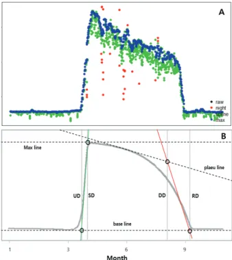
추출한 Gcc는 “Night, Spline, Max” 필터로부터 안개, 구 름, 눈, 비, 렌즈 이물질 등 맑지 않은 날씨의 이미지는 제거하였다[Figure 3 and 4(A)], autoFilter function, Filippa et al., 2015). Night filter는 0.2 Gcc 이하의 값들은 제거하 여 어둡거나 안개가 있는 이미지들을 필터링하였다. 나 쁜 날씨 조건, 낮은 광량, 더러운 렌즈와 같은 현상은 시계 열적 식생지수를 결정하는데 가장 흔한 문제들 중 하나이 다. Spline filter는 Gcc 값을 평활화(smoothing) 하였다 (Migliavacca et al., 2011). 마지막으로 Max filter는 Gcc 값을 3-day moving window 값을 산출하여 90% 이상의 값을 제거 하였다[Figure 4(A), Sonnentag, 2012]. 일반적 으로 Gcc 평확 곡선(curve fitting)하는 방법으로는 Gu et al.
(2009)의 방법에 따라 이중-로지스틱 함수(double-logistic function)로 Gcc 평활 곡선을 적용하였다(Figure 7).
Gcc 시계열에 대한 불확실성 함수는 관측된 데이터 점 주위에 균일한 잔차 분포를 생성한다. 이후 이중 로지스틱 적합치를 데이터(100번 반복)에 반복적으로 적용하였다.
Figure 3. Filters were applied to representative images.
Figure 4. Variations of phenophase analysis processing. A) Filtered relative greenness index. B) Illustration of the Gu method used to extract phenological thresholds (phenophases) in a seasonal Gcc trajectory (f’(t)).
반복 적용된 적합치에 대하여 식물계절 현상을 추출하였 다. 식물계절 현상 앙상블의 25번째 백분위수와 75번째 백분위수는 중앙값의 식물계절 현상 DOY (day of year) 주변의 신뢰 구간으로 사용된다(Figure 8). Gu et al.(2009) 의 방법에 의해 추출된 식물계절 현상은 UD (upturn date), SD (stabilization date), DD (downturn date), RD (recession date), GSL (growing season length)로 구분하였고, UD는 Gcc 값이 지속적으로 증가를 시작한 일, SD는 Gcc 최고값 의 일, DD는 Gcc 값이 지속적으로 감소를 시작한 일, RD 는 식물이 계절적으로 낮을 때, GSL은 UD부터 RD까지로 생장기간을 나타낸다[Figure 4(B), 5 and 8]. 식물계절 현 상을 구분하는 방법으로는 최소선(baseline)과 최대선 (maxline)은 Gcc의 최소값과 최대값에서 수평선을 생성하
Figure 5. Representative images and phenophase Gcc trajectory for phenological phase. The images represent the phenological timings of UD, SD, DD, and RD. UD: upturn date (Gcc begin to increase consistently), SD: stabilization date (maximum Gcc), DD: downturn date (Gcc starts to consistently diminish), RD:
recession date(vegetation reaches a seasonal low).
여, UD와 RD는 최소선과 최대선으로부터 봄철 식물의 생 장율과 노화율의 기울기에 의해 결정된다[Figure 4(B)]. Gcc 가 감소하는 성숙기간(SD-DD)은 성숙기선(plateau line)에 의하여 결정된다. 추출한 식물계절 현상의 정확도 검증에 는 RMSE (root mean square error)지수를 사용하였다. 추 출한 식물계절 현상의 정확도 검증에는 관측값의 불일치 도를 나타내기 위해 오차의 제곱근을 산술평균한 값의 제 곱근으로 예측의 전체적인 편향을 나타내는(Wald, 2002) RMSE (root mean square error)지수를 사용하였다(Jin et al., 2017).
결과 및 고찰
점봉산 신갈나무군락 내 상관우점종이 신갈나무인 두 구역(ROI1과 ROI2)과 소나무 한 구역(ROI3)을 대상으로
Figure 6. Seasonal patterns of color channel in region of interest (ROI)1 (a), ROI2 (b),and ROI3 (c) in Mt. Jeombong (left: raw digital number, right: relative index).
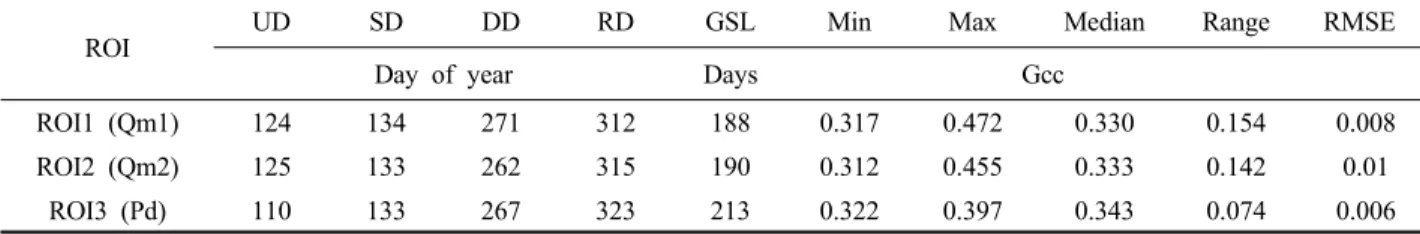
ROI UD SD DD RD GSL Min Max Median Range RMSE
Day of year Days Gcc
ROI1 (Qm1) 124 134 271 312 188 0.317 0.472 0.330 0.154 0.008
ROI2 (Qm2) 125 133 262 315 190 0.312 0.455 0.333 0.142 0.01
ROI3 (Pd) 110 133 267 323 213 0.322 0.397 0.343 0.074 0.006
Table 1. Summary of phenophase dates in regions of interest (ROIs): upturn date (UD), stabilization date (SD), downturn date (DD), recession date (RD), growing season length (GSL), annual minimum green chromatic coordinate (Gcc), annual maximum Gcc, annual median Gcc, and total range of Gcc.
ROI에 RGB DN을 추출하였다(Figure 6). ROI별 Red DN 평균은 141.77(ROI1), 133.74(ROI2), 124.82(ROI3) 순으로 나타났다. 상관우점종이 신갈나무인 ROI1과 ROI2는 낙엽 활엽수림으로 상록침엽수인 ROI3(상관우점종이 소나무) 에 비교하여 Red DN이 높게 나타났다. Green DN 평균은 Red DN 평균과 같은 순으로 142.85(ROI1), 137.00(ROI2), 131.12(ROI3) 순으로 나타났다.
ROI별 RGB DN을 Rcc, Gcc, Bcc로 산출하였다(Figure 6 and Table 1). ROI1의 Gcc 중앙값은 0.33으로 최소 0.317 과 최대 0.472로 나타났다. ROI2의 Gcc 중앙값은 0.333으 로 최소 0.312과 최대 0.455로 나타났다. ROI3의 Gcc 중앙 값은 0.343으로 최소 0.322과 최대 0.397으로 나타났다.
낙엽활엽수림과 상록침엽수림의 Gcc 진폭(Range)은 낙엽 활엽수림이 0.154와 0.142이며, 상록침엽수림은 0.074으 로 낙엽활엽수림의 Gcc 진폭의 크기가 상록활엽수림 보 다 크게 나타났다. 점봉산 상록침엽수림의 Gcc 진폭은 미 국 네바다주 아고산지역의 상록침엽수림(juniper forest)의 Gcc 진폭 크기와 유사하게 나타났다(Snyder et al., 2016).
또한 상록침엽수림은 낙엽활엽수림과 비교하여 Gcc의 증 가와 감소하는 기울기가 완만하게 나타났다. 이러한 결과 는 온대 낙엽활엽수림의 Gcc의 계절 특성을 연구한 결과 (Snyder et al., 2016; Toomey et al., 2015; Richardson, 2019)와 유사한 경향성을 보였다. 이는 본 연구의 데이터 가 일반적으로 상록침엽수림이 낙엽활엽수림에 비해 Gcc 의 계절적 진폭이 작은 특징(Hufkens et al., 2018)을 나타 내는 Gcc의 계절적 특성을 잘 반영하였다.
Figure 7은 ROI별 시계열 Gcc를 Gu et al.(2009) 따라 평활 곡선(curve fit)을 나타냈다. 소나무림(ROI3)은 신갈 나무림(ROI1과 ROI2) 보다 평활 곡선 궤적의 증가가 일찍 일어났으며, 감소 또한 일찍 일어났다. 봄철(DOY 60) 소 나무림(ROI3)은 Gcc 0.339부터 증가하여 여름철(DOY 152) Gcc 0.377로 최고치를 나타냈다. 반면에, 신갈나무림 (ROI1과 2)의 봄철과 가을철의 Gcc는 전반적으로 낮게 나 타났다. 봄철 신갈나무림(ROI1)의 Gcc가 0.328부터 증가 하여 여름철(DOY 152)에는 0.451로 최고치를 나타냈다.
Figure 7. Fitted curves for ROIs; Quercus mongolica canopy (blue line), Quercus mongolica canopy (red line), Pinus densiflora (green line).
또한 낙엽활엽수림(신갈나무림)인 ROI1과 ROI2의 식물 계절 현상의 패턴은 유사하였으나, 봄철 Gcc의 최대값은 ROI1이 더 높게 나타났다. 이는 디지털 카메라와 대상 구 역과의 거리차이에 의한 신갈나무 잎의 빛 반사 정도와 낙엽활엽수가 분포하고 있는 위치(ROI1은 능선 및 북사면 과 ROI2는 남사면)에 의하여 Gcc 최대값의 차이를 보인 것으로 사료된다.
점봉산 신갈나무군락의 상관우점종 으로부터 구획된 ROIs의 식물계절적 현상(phenophase)을 UD, SD, DD, RD, GSL로 구분하였다(Table 1 and Figure 8). ROI1의 UD는 DOY 124로 ROI2의 DOY 125와 1일의 차이를 보였고, RD는 ROI1이 DOY 312로 ROI2는 DOY 315와 3일의 차 이를 보였다. GSL(식물의 생장기간)은 ROI1이 188일 이 며 ROI2는 190일로 나타났다.
추출한 식물계절 현상의 정확도는 RMSE 값이 0.05 미 만 이여야 정확도가 높다고 판단할 수 있다(Chai and Draxler, 2014; Jin et al., 2017). 식물계절 현상의 정확도는 RMSE가 0.008(ROI1)과 0.006(ROI3)으로 높은 정확도를
Figure 8. Uncertainty estimation applied to the Gcc trajectory in the forest ecosystem, Mt. Jeombong. The grey lines represent the 100 simulated curves on which phenophases are extracted. The images of a, b, c and d represent the phenological timings of UD, SD, DD, and RD. UD: upturn date (Gcc begin to increase consistently), SD: stabilization date (maximum Gcc), DD: downturn date (Gcc starts to consistently diminish), RD: recession date (vegetation reaches a seasonal low).
나타냈다. 높은 정확도를 나타낸 ROI1과 3의 식물계절 현 상을 나타냈다(Figure 8). 소나무림(ROI3)의 UD와 RD는 각각 DOY 110과 323으로 나타났으며, 생장기간은 213일 로 나타났다. 소나무림과 신갈나무림의 식물계절적 특징 으로는 소나무림은 생장의 시작(UD)이 신갈나무림에 비 하여 빨랐고, 생장의 종료(RD)는 늦은 것으로 나타났다.
생장기간 또한 213일로 신갈나무에 비하여 길게 나타났 다. Jang et al.(2020)은 2010년부터 2018년까지의 가야산 소나무(해발고도 1,180 m)와 신갈나무(해발고도 1,300 m) 의 개엽 시작일(UD)은 각각 134.1일과 123.7일로 보고하 였다. 이는 본 연구결과의 신갈나무 UD DOY와 일치하는 것으로 나타났다. 하지만 소나무는 약 24일의 차이를 보였 다. 이러한 차이점은 직접 사람에 의하여 현장에서 수행하 는 식물계절 조사방법의 상록침엽수 개엽 시작일 기준과 (새롭게 생성된 줄기 중 처음 잎눈이 터져 잎다발이 보이 기 시작할 때)과 이미지를 활용한 식물계절 현상 파악 방 법의 개엽 시작일 기준(Gcc 값이 지속적으로 증가를 시작 한 일)이 다르기 때문인 것으로 사료된다.
결 론
본 연구에서는 전통적인 현장조사와 위성영상을 이용한 식물계절 관찰의 한계를 극복하기 위하여 점봉산 산림생 태계의 경관을 디지털 카레라로 촬영된 고해상도 및 고빈 도 반복 이미지를 이용하여 식물계절 변화 관찰 방법을 국내에 적용 가능성을 진단하였고, 식물계절 변화 관찰과
계절변화 현상을 정량화하였다. 도출된 식물계절 데이터 및 분석으로부터 온대중부 낙엽활엽수림의 특성에 따른 식물의 계절 경향성을 분석하였다. 상록침엽수림은 낙엽 활엽수림과 비교하여 Gcc의 진폭의 크기가 작았으며, 봄 철과 가을철의 기울기 또한 완만하였다. 이러한 특성은 국 외의 온대 낙엽활엽수림과 상록침엽수림의 계절적 Gcc 특성과 유사하였다. 낙엽활엽수인 ROI1과 ROI2의 식물계 절 현상의 패턴은 유사하였으나, 봄철 Gcc의 최대값은 ROI1이 더 높게 나타났다. 이는 디지털 카메라와 대상 구 역과의 거리차이에 의한 신갈나무 잎의 빛 반사 정도와 낙엽활엽수가 분포하고 있는 위치에 의하여 Gcc 최대값 의 차이를 보인 것으로 사료된다. 소나무림과 신갈나무림 의 식물계절적 특징으로는 소나무림은 생장의 시작(UD) 이 신갈나무림에 보다 빨랐고, 생장의 종료(RD)는 늦은 것으로 나타났다. 생장기간 또한 213일로 신갈나무림에 비하여 길게 나타났다. 이를 전통적인 식물계절 조사방법 으로 관찰된 계절변화 현상과 비교하였을 때 신갈나무림 의 개엽 시작일(UD)은 일치하였지만, 소나무림은 약 24일 의 차이를 보였다. 이는 식물계절 현상의 기준을 나눌 때 반복 이미지 식물계절 현상 관측과 전통적 현장조사 방법 에서의 상록침엽수림의 개엽 시작일을 정의하는 기준이 다르기 때문인 것으로 사료된다.
산림생태계에 디지털 카메라의 설치와 ‘phenopix’ packages 분석으로부터 도출된 본 연구의 데이터는 온대북부형 낙 엽활엽수림에서 나타나는 Gcc 궤적과 식물계절 특성을 잘 반영하였다. 하지만 향후 전통적인 식물계절 실측 자료
와 위성영상으로부터 반복 이미지의 식물계절 현상 분석 에 보완 및 검증 자료가 필요할 것으로 사료된다. 또한 기후에 따른 식물의 계절변화와의 상관관계를 파악하고, 현재 군락수준의 관측에서 위성영상 자료를 통한 지역 또 는 국가수준의 식물계절 변화현상 연구가 진행되어야 할 것이다.
감사의 글
본 연구는 국립생태원 ‘생태계 기후변화 조사 연구(NIE- 기반연구-2020-21)’의 지원으로 이루어진 것입니다.
References
Ahas, R. and Aasa, A. 2006. The effects of climate change on the phenology of selected Estonian plant, bird and fish populations. International Journal of Biometeorology 51(1): 17-26.
Ahrends, H.E., Etzold, S., Kutsch, W.L., Stöckli, R., Brügger, R., Jeanneret, F., Wanner, H., Buchmann, N. and Eugster, W. 2009. Tree phenology and carbon dioxide fluxes: use of digital photography for process-based interpretation at the ecosystem scale. Climate Research 39(3): 261-274.
Alberton, B., Almeida, J. Helm, R. Torres, R.S., Menzel, A.
and Morellato, L.P. 2014. Using phenological cameras to track the green up in a cerrado savanna and its on-the- ground validation. Ecological Informatics 19: 62-70.
Alberton, B., Torres, R.S., Cancian, L.F., Borges, B.D., Almeida, J., Mariano, G.C., Santos, J. and Morellato, L.P.C.
2017. Introducing digital cameras to monitor plant phenology in the tropics: applications for conservation.
Perspectives in Ecology and Conservation 15(2): 82-90.
Baghzouz, M., Devitt, D.A., Fenstermaker, L.F. and Young, M.H. 2010. Monitoring vegetation phenological cycles in two different semi-arid environmental settings using a ground-based NDVI system: A potential approach to improve satellite data interpretation. Remote Sensing 2(4):
990-1013.
Brown, T.B., Hultine, K.R., Steltzer, H., Denny, E.G., Denslow, M.W., Granados, J., Henderson, S., Moore, D., Nagai, S.
and SanClements, M. 2016. Using phenocams to monitor our changing Earth: toward a global phenocam network.
Frontiers in Ecology and the Environment 14(2): 84-93.
Chai, T. and Draxler, R.R. 2014. Root mean square error (RMSE) or mean absolute error (MAE)?-Arguments against avoiding RMSE in the literature. Geoscientific Model development 7(3): 1247-1250.
Choi, C.H., Jung, S.G. and Park, K.H. 2016. Analysing relation- ship between satellite-based plant phenology and temper- ature. Journal of the Korean Association of Geographic Information Studies 19(1): 30-42.
Crick, H.Q., Dudley, C., Glue, D.E. and Thomson, D.L. 1997.
UK birds are laying eggs earlier. Nature 388(6642):
526-526.
Filippa, G., Cremonese, E., Galvagno, M., Migliavacca, M., Di Cella, U.M., Petey, M. and Siniscalco, C. 2015. Five years of phenological monitoring in a mountain grassland:
inter-annual patterns and evaluation of the sampling protocol. International journal of biometeorology 59(12):
1927-1937.
Fisher, J.I., Mustard, J.F. and Vadeboncoeur, M.A. Green leaf phenology at Landsat resolution: Scaling from the field to the satellite. Remote Sensing of Environment 100(2):
265-279.
Garrity, S.R., Vierling, L.A. and Bickford, K. 2010. A simple filtered photodiode instrument for continuous measurement of narrowband NDVI and PRI over vegetated canopies.
Agricultural and Forest Meteorology 150(3): 489-496.
Graham, E.A., Riordan, E.C., Yuen, E.M., Estrin, D. and Rundel, P.W. 2010. Public Internet‐connected cameras used as a cross‐continental ground‐based plant phenology moni- toring system. Global Change Biology 16(11): 3014-3023.
Gu, L., Post, W.M., Baldocchi, D.D., Black, T.A., Suyker, A.E., Verma, S.B, Vesala, T. and Wofsy, S.C. 2009.
Characterizing the seasonal dynamics of plant community photosynthesis across a range of vegetation types.
Phenology of Ecosystem Processes. Springer 35-58.
Hufkens, K., Filippa, G., Cremonese, E., Migliavacca, M., D'Odorico, P., Peichl, M., Gielen, B., Hörtnagl, L., Soudani, K., Papale, D., Rebmann, C., Brown, T. and Wingate, L. 2018. Assimilating phenology datasets automatically across ICOS ecosystem stations. Agricultural and Forest Meteorology 249: 275-285.
Ide, R. and Oguma, H. 2010. Use of digital cameras for pheno- logical observations. Ecological Informatics 5(5): 339-347.
IPCC (Intergovernmental Panel on Climate Change). 2018.
Summary for Policymakers. In: Global Warming of 1.5°C.
World Meteorological Organization. Switzerland pp. 32.
Jang, J.G., Yoo, S.T., Kim, B.D., Son, S.W. and Yi, M.H.
2020. The Relationship Between Temperature and Spring Phytophenological Index. Korean Journal of Plant Resources 33(2): 106-115.
Jin, Y.H., Zhu, J.R., Sung, S.Y. and Lee, D.K. 2017.
Application of satellite data spatiotemporal fusion in predicting seasonal NDVI. Korean Journal of Remote Sensing 33(2): 149-158.
Kim, H.J., Hong, J.K., Kim, S.C., Oh, S.H. and Kim, J.H.
2011. Plnat phenology of threatened species for climate change in sub-alpine zone of Korea. Korea Journal of Plant Resources 24(5): 549-556.
Kim, H.W. 2019. Changes of the flowering time of tree in spring by climate change in Seoul, South Korea. Seoul.
Ewha Womans University.
Kurc, S.A. and Benton, L.M. 2010. Digital image-derived greenness links deep soil moisture to carbon uptake in a creosotebush-dominated shrubland. Journal of Arid Environments 74(5): 585-594.
Lee, B.R., Kim, E.S., Lee, J.S., Chung, J.M. and Lim, J.H.
2018. Detecting phenology using MODIS vegetation indices and forest type map in South Korea. Korean Journal of Remote Sensing 34(2-1): 267-282.
Lee, K.M., Kwon, W.T. and Lee, S.H. 2009. A study on plant phenological trends in South Korea. Journal of The Koraen Association of Regional Geographers 15(2): 337-350.
Menzel, A. 2000. Trends in phenological phases in Europe between 1951 and 1996. International Journal of Bio- meteorology 44(2): 76-81.
Migliavacca, M., Galvagno, M., Cremonese, E., Rossini, M., Meroni, M., Sonnentag, O., Cogliati, S., Manca, G., Diotri, F. and Busetto, L. 2011. Using digital repeat photography and eddy covariance data to model grassland phenology and photosynthetic CO2 uptake. Agricultural and Forest Meteorology 151(10): 1325-1337.
Morellato, L.P.C., Alberton, B., Alvarado, S.T., Borges, B., Buisson, E., Camargo, M.G.G., Cancian, L.F., Carstensen, D.W., Escobar, D.F. and Leite, P.T. 2016. Linking plant phenology to conservation biology. Biological Conservation 195: 60-72.
Morisette, J.T., Richardson, A.D., Knapp, A.K., Fisher, J.I., Graham, E.A., Abatzoglou J., Wilson, B.E., Breshears, D.D., Henebry, G.M., Hanes, J.M. and Liang, L. 2008.
Tracking the rhythm of the seasons in the face of global change: phenological research in the 21st century. Frontiers in Ecology and the Environment 7(5): 253-260.
Moulin, S., Kergoat, L., Viovy, N. and Dedieu, G. 1997. Global- Scale Assessment of Vegetation Phenology Using NOAA/
AVHRR Satellite Measurements. Journal of Climate 10(6):
1154-1170.
Parry, M.L., Canziani, O.F., Palutikof, J.P., Linden, P.J. and Hanson, C.E. 2007. Climate Change 2007: Impacts, Adaptation, and Vulnerability. Cambridge University Press pp. 939.
Pau, S., Wolkovich, E.M., Cook, B.I., Davies, T.J., Kraft, N.J.B., Bolmgren, K., Betancourt, J.L. and Cleland, E.E.
2011. Predicting phenology by integrating ecology, evolu-
tion and climate science. Global Change Biology 17(12):
3633-3643.
Petach, A.R., Toomey, M., Aubrecht, D.M. and Richardson, A.D. 2014. Monitoring vegetation phenology using an infrared-enabled security camera. Agricultural and forest meteorology 195: 143-151.
Pettorelli, N., Vik, J.O., Mysterud, A., Gaillard, J.M., Tucker, C.J. and Stenseth, N.C. 2005. Using the satellite-derived NDVI to assess ecological responses to environmental change. Trends in Ecology & Evolution 20(9): 503-510.
Polgar, C.A. and Primack, R.B. 2011. Leaf‐out phenology of temperate woody plants: from trees to ecosystems. New Phytologist 191(4): 926-941.
R-Forge Phenopix. https://r-forge.r-project.org/projects/phenopi/.
(2020.06.04.).
Richardson, A.D. 2019. Tracking seasonal rhythms of plants in diverse ecosystems with digital camera imagery. New Phytologist 222(4): 1742-1750.
Richardson, A.D., Braswell, B.H., Hollinger, D.Y., Jenkins, J.P. and Ollinger, S.V. 2009. Near‐surface remote sensing of spatial and temporal variation in canopy phenology.
Ecological Applications 19(6): 1417-1428.
Richardson, A.D., Jenkins, J.P., Braswell, B.H., Hollinger, D.Y., Ollinger, S.V. and Smith, M.L. 2007. Use of digital webcam images to track spring green-up in a deciduous broadleaf forest. Oecologia 152(2): 323-334.
Richardson, A.D., Keenan, T.F., Migliavacca, M., Ryu, Y., Sonnentag, O. and Toomey, M. 2013. Climate change, phenology, and phenological control of vegetation feed- backs to the climate system. Agricultural and Forest Meteorology 169: 156-173.
Ryu, Y., Baldocchi, D.D., Verfaillie, J., Ma, S., Falk, M., Ruiz- Mercado, I., Hehn, T. and Sonnentag, O. 2010. Testing the performance of a novel spectral reflectance sensor, built with light emitting diodes (LEDs), to monitor ecosystem metabolism, structure and function. Agricultural and Forest Meteorology 150(12): 1597-1606.
Scrantona, K. and Amarasekarea, P. 2017. Predicting pheno- logical shifts in a changing climate. Proceedings of the National Academy of Sciences of the United States of America 114(50): 13212-13217.
Snyder, K.A., Wehan, B.L., Filippa, G., Huntington, J.L., Stringham, T.K. and Snyder, D.K. 2016. Extracting plant phenology metrics in a great basin watershed: Methods and considerations for quantifying phenophases in a cold desert. Sensors 16(11): 1948.
Sonnentag, O. Detto, M., Vargas, R., Ryu, Y., Runkle, B.R.K., Kelly, M. and Baldocchi, D.D. 2011. Tracking the struc- tural and functional development of a perennial pepper-
weed (Lepidium latifolium L.) infestation using a multi- year archive of webcam imagery and eddy covariance mea- surements. Agricultural and Forest Meteorology 151(7):
916-926.
Sonnentag, O., Hufkens, K., Teshera-Sterne, C., Young, A.M., Friedl, M., Braswell, B.H., Milliman, T., O’Keefe, J. and Richardson, A.D. 2012. Digital repeat photography for phenological research in forest ecosystems. Agricultural and Forest Meteorology 152: 159-177.
Tan B., Morisette J.T., Wolfe, R.E., Gao, F., Ederer, G.A., Nightingale, J. and Pedelty, J.P. 2011. An enhanced TIMESAT algorithm for estimating vegetation phenology metrics from MODIS data. IEEE Journal of Selected Topics in Applied Earth Observations and Remote Sensing 4(2):
361-371.
Tooke F. and Battey, N.H. 2010. Temperate flowering phenology.
Journal of Experimental Botany 61(11): 2853-2862.
Toomey, M., Friedl, M.A., Frolking, S., Hufkens, K., Klosterman, S., Sonnentag, O., Baldocchi, D.D., Bernacchi, C.J., Biraud, S.C. and Bohrer, G. 2015. Greenness indices from digital cameras predict the timing and seasonal dynamics of canopy-scale photosynthesis. Ecological Applications 25(1): 99-115.
Ulsig, L., Nichol, Caroline J., Huemmrich, K.F., Landis, D.R., Middleton, E.M., Lyapustin, A.I., Mammarella, I., Levula, J. and Porcar-Castell, A. 2017. Detecting inter-annual variations in the phenology of evergreen conifers using long-term MODIS vegetation index time series. Remote sensing 9(1): 49.
Wald, L. 2002. Data fusion: definitions and architectures: fusion of images of different spatial resolutions. Les Presses del'É
cole des Mines. Paris. pp. 198.
Whitfield, J. 2001. The budding amateurs. Nature 414: 578-579.
WMO (World Meteorological Organization). 2019. WMO statement on the state of the global climate in 2019.
WMO-No. 1248: 1-44.
Zhang, X., Friedl, M.A., Schaaf, C.B., Strahler, A.H., Hodges, J.C.F., Gao, F., Reed, B.C. and Huete, A. 2003. Monitoring vegetation phenology using MODIS. Remote Sensing of Environment 84(3): 471-475.
Manuscript Received : August 12, 2020 First Revision : October 27, 2020 Second Revision : November 29, 2020 Accepted : November 30, 2020