Noncontact Fatigue Crack Evaluation Using Thermoelastic Images

(1)

Noncontact Fatigue Crack Evaluation Using Thermoelastic Images

Ji-Min Kim*, Yun-Kyu An* and Hoon Sohn*^✝

Abstract This paper proposes a noncontact thermography technique for fatigue crack evaluation under a cyclic tensile loading. The proposed technique identifies and localizes an invisible fatigue crack without scanning, thus making it possible to instantaneously evaluate an incipient fatigue crack. Based on a thermoelastic theory, a new fatigue crack evaluation algorithm is proposed for the fatigue crack-tip localization. The performance of the proposed algorithm is experimentally validated. To achieve this, the cyclic tensile loading is applied to a dog-bone shape aluminum specimen using a universal testing machine, and the corresponding thermal responses induced by thermoelastic effects are captured by an infrared camera. The test results confirm that the fatigue crack is well identified and localized by comparing with its microscopic images.

Keywords: Fatigue Crack Detection, Thermoelastic Effects, Nondestructive Evaluation, Noncontact Thermography

[Received: November 7, 2012, Revised: December 10, 2012, Accepted: December 12, 2012] *Department of Civil and Environmental Engineering, KAIST, 373-1, Guseong-dong, Yuseong-gu, Deajeon 305-701, Korea ✝Corresponding Author: [email protected]

1. Introduction

Fatigue crack detection has become a critical issue in nondestructive evaluation (NDE) com- munity because a fatigue crack may cause catastrophic failure of a structure. The structures under the repetitive loadings are vulnerable to a fatigue crack produced by a stress even less than the fracture limit. Since the incipient fatigue crack is often closed, its invisibility makes it more difficult to detect in early stage.

Many researchers have investigated fatigue crack detection using various NDE techniques. Klepka et al. and Quan et al. utilized a nonlinear acoustic method to detect a fatigue crack [1,2].

However, acoustical nonlinearity may come from the intrinsic nonlinear properties of a target material and testing equipments, thus leading to false alarms. Moreover, fatigue crack localization and precise quantification using the nonlinear acoustic method are very challenging work. Another widely used NDE technique is eddy current techniques. Peng et al. developed a novel eddy current probe for fatigue crack

detection and Liu et al. estimated the location of surface cracks on aircraft tubes by using an eddy current array instrument [3,4]. Then, magnetic flux also has been used for fatigue crack detection. Tanabe et al. estimated a fatigue crack on a steel specimen by measuring the magnetic flux density around a fatigue crack- tip [5,6]. Although both techniques give reliable results for fatigue crack detection, their working distances are quite limited. Thus, it is hard to apply these techniques to real structures under in-service loading conditions.

In recent years, thermography techniques have been proposed for fatigue crack detection.

They have the following advantages compared to other NDE techniques: (1) noncontact, (2) full-field measurement, (3) intuitive damage diagnosis and (4) long working distance.

The thermography technique is classified into

"active" and "passive" techniques. The "active thermography" observes thermal changes of a target structure using external actuating sources.

For the crack detection, several active

thermography techniques such as ‘eddy current

(2)

thermography’, ‘laser thermography’ and

‘vibrothermography’ have been proposed and proved their capabilities.

The eddy current thermography produces a current flow on a target surface by the induction effect of coils near the surface and observes the heat blocking by an existing fatigue crack [7].

Cheng et al. studied to detect a surface- breaking crack on a CFRP material used in aircraft and wind turbine blades [8]. Then, the laser thermography utilizes a laser source to generate heat flow and similarly measures the heat blocking effect by a crack. Li et al.

showed its capability to evaluate a micro fatigue crack and Schlichting et al. estimated the crack size and depth not only location [9,10]. Since this laser thermography is capable of an inspection at the long distance, it is potentially valuable approach for real applications. The vibrothermography detects a fatigue crack by capturing the heat generated by friction at crack interface, when the energy of ultrasonic waves causes crack surfaces to rub [11,12]. Morbidini et al. has examined the capability of the vibro- thermography for fatigue crack detection on mild steel and nickel-based superalloy specimens [13].

Recently, the vibrothermography-based automated crack detection algorithm was proposed by Li et al. [14]. Although various active thermography techniques for fatigue crack detection have been successfully proven in structures under static state condition, they are still limited to be applied to in-service structures.

On the other hand, the passive thermography records thermal signals emitted from a structure itself without any external actuating energy [15].

Since it does not need any external actuating source and contact, it has a clear advantage in evaluating a crack under in-service condition of a target structure.

A thermoelastic stress analysis (TSA) has been studied as one of the representative passive techniques [16-18]. It builds on the ‘thermo-

elasctic effects’ which are temperature changes caused by force-induced volume changes [19].

TSA provides stress fields around a crack-tip and predicts the fatigue life by measuring the thermoelastic signals. The thermoelastic effects offer a chance to evaluate a fatigue crack.

In this paper, a new fatigue crack evaluation algorithm based on the thermoelastic images obtained by using an infrared camera is proposed and experimentally validated. The proposed algorithm has following advantages:

(1) intuitive fatigue crack identification with low computational cost, (2) instantaneous and robust crack diagnosis without any baseline data previously obtained from a pristine condition of the structure and (3) precise crack length estimation.

This paper is organized as follows. First, the proposed algorithm is explained in section 2.

Then, the experimental setup for a fatigue crack evaluation test on a dog-bone shape aluminum plate is described in section 3. Section 4 discusses the performance of the proposed algorithm by comparing the estimated crack length with microscope images.

2. A Fatigue Crack Evaluation Algorithm Using Thermoelastic Images

2.1 Theoretical Background of the Thermoelastic Stress Analysis (TSA)

TSA utilizes thermoelastic signals caused by

thermoelastic effects that generally occur around

the crack-tip region during the cyclic loading to

estimate the stress status. The thermoelastic

effects state that temperature is changed due to

material volume change caused by an external

force. A compression force causes a temperature

increase, whereas a tensile force produces a

temperature decrease. From this effects, the

relationship between the thermoelastic signal and

the corresponding stress status can be expected

(3)

Fig. 1 Fatigue crack evaluation algorithm

and is given by [20] :

∆_ _ 

 (1)

where the σ

¹

and σ

²

are the principal stresses and the A and S indicate the calibration factor and the magnitude of the measured thermoelastic signal, respectively.

Eq. (1) assures that it’s very attractive to use TSA for a fatigue crack evaluation, because stress concentration around a crack-tip can be estimated by simply measuring thermoelastic signals at the target surface.

2.2 A Fatigue Crack Evaluation Algorithm In this subsection, a new fatigue crack evaluation algorithm using the thermoelastic images obtained from a structure under cyclic loading condition is explained. The proposed algorithm aims to localize a crack-tip and precisely estimate the fatigue crack length.

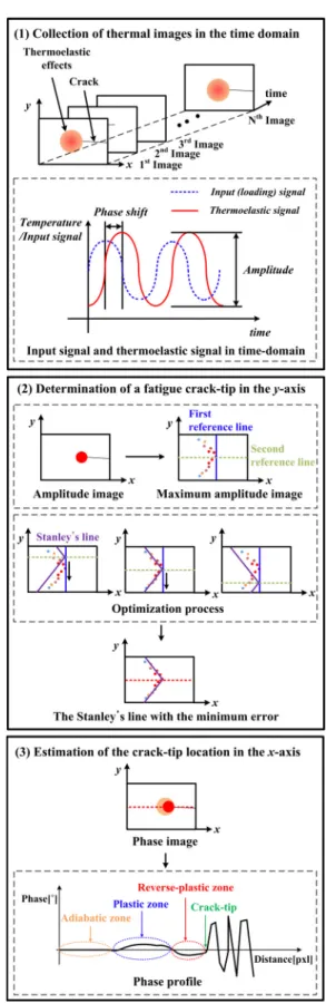
Fig. 1 shows the procedure of the fatigue crack evaluation algorithm. The details of each step are as follows:

(1) As shown in the first part of Fig. 1, the thermal images of an inspection area are captured and stored by an infrared camera.

Thermoelastic signal at each pixel of the thermal images in the time domain is processed to acquire the “amplitude image” and the “phase image”.

A set of the amplitude of the thermoelastic signal at each pixel produces the “amplitude image” showing how much stress is applied to.

Then, the “phase image” represents the amount

of the phase shift compared to the input signal

which is identical to the loading signal applied

to a structure. Progression of the plastic work

makes the adiabatic condition no longer hold. In

plastic region, it brings about the heat

dissipation which leads to the phase shift of the

thermoelastic signal compared to the input

signal [21]. Depending on how much the plastic

(4)

work has been progressed, the amount of the phase shift is assigned to each pixel. The phase difference between the input signal and the thermoelastic signal at each pixel produces the

“phase image”.

(2) Stanley’s methodology, which is an experimental observation presenting the relationship between the crack orientation and maximum thermoelastic signals of each line parallel to the crack orientation, is employed as a theoretical basis in this study [22]. It is deduced by the measured thermoelastic signals and the Westergaard’s model describing the stress status at the corresponding pixel in the region where the linear elastic relation is achieved between the thermoelastic signal and the stress status. This model is expressed as follows [23]:

∆_ _  



^

∆



_

  

  



^

∆



_

 



(2) where the ‘

^∆



_

’ and ‘

^∆



_

’ are the stress intensity factors (SIFs) for Mode I and Mode II loading respectively, the ‘r’ is the distance from the crack-tip and the ‘

^

’ is the angle between the crack orientation and the line connecting the corresponding point and the crack-tip. According to the Stanley’s observation, for the pure Mode I fatigue loading, the maximum thermoelastic signal at any line parallel to an existing crack occurs at 60 degrees with respect to the crack orientation [22].

In this paper, the loading condition is restricted to a pure Mode I loading by applying uniaxial tensile loads. Under this assumption, the crack propagation direction is perpendicular to the loading axis. Thus, the maximum thermo- elastic signals maintain 60 degrees with respect to the crack propagation direction.

The second part of Fig. 1 shows procedures to determine a fatigue crack-tip in y-axis. To utilize the Stanley’s observation, first the

“maximum amplitude image” is produced by picking up all of the maximum thermoelastic signals at each line perpendicular to the loading axis. The data distribution of the maximum thermoelastic signals of the maximum amplitude image shows the trend that the Stanley stated in his observation. From this result, although the Stanley’s observation enables to estimate the crack-tip location in the y-axis intuitively, several factors such as noise components and unreliable judgement of users may produce considerable error. Thus, an optimization process is required to determine more reliable and robust crack-tip location in the y-axis.

As the first step of the optimization process based on the maximum amplitude image, three components are defined: two reference lines and the Stanley’s line.

In advance, the first reference line is defined as the parallel line to the loading axis across the maximum point of the maximum amplitude image which is considered as the closest point to the crack-tip by the Eq. (1) and (2). It divides the inspection area into two regions, i.e.

the thermoelasticity region and the crack region.

In general, since the applied stress in the thermoelasticity region is larger than that in the crack region, the maximum thermoelastic signals of the maximum amplitude image exist in the thermoelasticity region. Then, the second reference line is drawn at an arbitrary point of the first reference line. The two reference lines are perpendicular to each other and the second reference line is parallel to the crack orientation.

At the intersection of the first and second

reference line, two straight lines are drawn

towards the thermoelasicity region defined by

the first reference line. They maintain 60

degrees with respect to the second reference line

and are defined as “Stanley’s line”. During

the optimization process, the second reference

line and the Stanley’s line change their position

from the top to bottom position of the first

(5)

reference line.

On the basis of those three components, now the error function for this optimization process is defined as follows:



 



  



_ _^

(3)

where n is the step number of the second reference line, the m

i

and s

i

are the distance from the first reference line to the maximum thermoelastic signal and the Stanley’s line, respectively. The calculated value from the Eq. (3) is the index indicating how well each Stanley’s line is correlated with the maximum thermoelastic signal and which is the best Stanley’s line with the minimum error.

As the position of the second reference line changes along the first reference line, the error is calculated by the Eq. (3) for each step. When the minimum value is obtained, the y-coordinate of the second reference line is equivalent to that of the crack-tip.

(3) The crack-tip location in the x-axis is determined by the phase analysis. As shown in the third part of Fig. 1, the phase profile of the second reference line determined at the previous stage is extracted from the phase image. It is divided into three different regions: adiabatic zone, plastic zone and reverse-plastic zone [21].

For the effective image processing, it is supposed that input signal and the thermoelastic signal of the adiabatic zone are in-phase, which means there is no phase difference in the adiabatic zone. Before the plastic work of the material, whole inspection area is considered achieving the adiabatic condition. However, as the plastic work induced by the external cyclic loading causes heat dissipation leading to the phase shift, the phase difference in the plastic region has positive values. Phase profile shows that, at the very close region to the crack-tip, there exists the reverse-plastic zone where the stress is applied to the opposite direction of the

plastic zone. Therefore, the sign of the phase difference is reversed to the negative. After the reverse-plastic zone, the phase profile fluctuates randomly because of the arbitrary radiation from the background light coming through an opening between crack interface. Here, the point where the sign of the phase profile changes from negative to positive is defined as the crack-tip location which is the transient point from the reverse-plastic zone to the random fluctuation.

Through the optimization process of the Stanley’s observation and the phase analysis, the crack-tip is identified and localized. The crack-tip location is used to estimate a crack length. A perpendicular line is determined crossing a notch-tip location and a vertical distance between this line and the determined crack-tip location is defined as the estimated crack length.

3. Experimental Setup

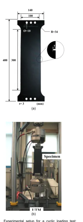
To validate the performance of the proposed fatigue crack evaluation algorithm, a dog-bone shape aluminum plate is prepared which is coated by black paint to increase emissivity and maintain its consistency as shown in Fig. 2(a).

The notch of 5 mm long and 1 mm wide is produced at the center of the plate for the stress concentration at the notch-tip.

For the pure Mode I loading, the universal testing machine (INSTRON, 8801) is used. To achieve a cyclic tensile loading, the minimum and maximum amplitude is set to 1.4 kN and 14 kN. As a loading function, the sine function was used with the frequency 10 Hz until 135,000 cycles.

During the fatigue testing, the thermal

images are captured by the infrared camera

(InfraTEC, VarioCAM hr) with its spectral range

from 7.5 μm to 14 μm. Its geometric and

thermal resolution are 640 × 480 pixels and

0.03 K at 30 ℃, respectively. The sampling

(6)

(a)

(b)

Fig. 2 Experimental setup for a cyclic loading test:

(a) a dog-bone shape aluminum plate and (b) universal testing machine(UTM)

(a)

(b)

Fig. 3 Average crack width estimated by the microscopic images: (a) 43.8 μm at the notch-tip and (b) 5.3 μm at the crack-tip

frequency is set to 50 Hz and sensing distance is 500 mm from the aluminum plate.

The created micro fatigue crack is observed by a microscope. As shown in Fig. 3, the crack width are measured at both notch-tip and

crack-tip. The average crack width is 43.8 μm at the notch-tip and 5.3 μm at the crack-tip, respectively. The estimated crack length by a microscope is 14.55 mm which is used as the reference value to validate the performance of the proposed fatigue crack evaluation algorithm.

4. Results

In general, two factors are considered as a source of a heat generation around a crack. One is the thermoelastic effect around a crack-tip and the other is the friction between crack interface.

For the pure Mode I loading assumed in this

experiment, the thermoelastic effect by the stress

concentration at a crack-tip is expected as the

major factor of produced heat [12]. During the

fatigue testing, the range of the applied load set

in the tensile state (from 1.4 kN to 14 kN)

assures that the contact area is small enough so

that the friction-induced heat is minimized.

(7)

(a)

(b)

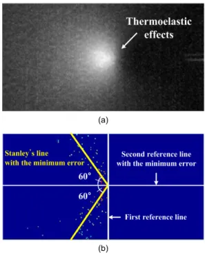
Fig. 4 Determination of the crack-tip location in the y-axis: (a) amplitude image and (b) the maximum amplitude image and the Stanley’s line with the minimum error

(a)

(b)

Fig. 5 Estimation of the crack-tip location in the x-axis through the phase profile: (a) phase image and (b) the phase profile of the second reference line with the minimum error

Therefore, the effect of the frictional heat is ignored and the captured thermal images are analyzed on the basis of TSA under the assumption that the thermoelastic effect is the main component of the produced heat around a crack.

The thermoelastic images acquired right before the end of the fatigue test are processed by the proposed fatigue crack evaluation algorithm so that the crack length at the end of the fatigue testing is precisely estimated without further crack propagation. From the amplitude image in Fig. 4(a), the thermoelastic effects around the crack-tip region can be observed.

According to the thermoelastic theory, it means that the stress concentration happens around the crack-tip region leading to a fatigue crack propagation.

The optimization process is applied to maximum thermoelastic signals of the maximum amplitude image. Along the first reference line, the second reference line and the Stanley’s line move and the defined error function calculates the error for each step. Optimization process determines the best Stanley’s line and the corresponding second reference line with the minimum error as shown in Fig. 4(b). The position of the second reference line in the y-axis indicates that of the crack-tip.

Fig. 5 shows the determination process of

the crack-tip location in the x-axis based on the

phase analysis. Fig. 5(a) is the phase image and

the dotted line indicates the second reference

line with the minimum error determined by the

optimization process. In Fig. 5(b), the phase

profile of the dotted line is shown and the

adiabatic zone and the reverse-plastic zone can

be clearly observed. However, the distinction of

the plastic zone is difficult which is supposed to

exist between two zones. In fact, the stress

concentration in the plastic zone is very little

compared to that in the reverse-plastic zone,

thus the lack of the thermal resolution of the

(8)

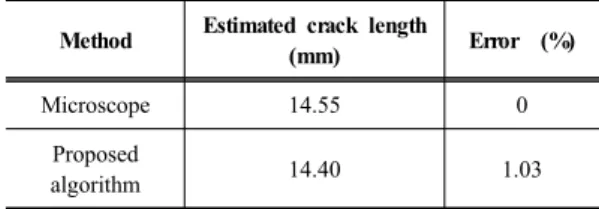
Table 1 Comparison of the estimated fatigue crack lengths

Method Estimated crack length

(mm) Error (%)

Microscope 14.55 0

Proposed

algorithm 14.40 1.03

infrared camera restricts to measure the small amount of thermoelastic signal change.

Moreover, the coating layer on the surface of the aluminum plate may disturb the accurate measurement of the thermoelastic signal, thus making it difficult to classify the plastic zone.

The crack-tip is located at the end of the reverse-plastic zone where the phase profile changes from negative to positive.

Based on the determined crack-tip location, the fatigue crack length is estimated. At section 2, a vertical distance from a crack-tip location to a perpendicular line crossing a notch-tip location is defined as a crack length and the crack length is estimated by determining the corresponding pixel number. The value of the

‘length/pixel’ is calculated as 0.45 mm/pixel and the estimated crack length is 14.40 mm.

5. Conclusion

This paper proposes a fatigue crack evaluation algorithm based on the thermoelastic images. The thermoelastic effects on the surface of a structure is analyzed by employing the Stanley’s observation and the phase analysis.

Main advantages of the proposed fatigue crack evaluation algorithm are (1) intuitive fatigue crack identification with low com- putational cost, (2) instantaneous and robust crack diagnosis without any baseline data previously obtained from a pristine condition of the structure and (3) precise crack length estimation.

The performance validation is attempted by estimating the fatigue crack length created on the dog-bone shape aluminum plate under the cyclic tensile loading until 135,000 cycles. The result is compared with the estimated fatigue crack length by a microscope in Table 1. The error percentage is 1.03 %, which represents the high detectability and robustness of the proposed fatigue crack evaluation algorithm.

Successful fatigue crack evaluation of the simple plate structure presents the possibility to apply the proposed algorithm to a more complex structure. In the future research, the applicability of the proposed algorithm to structures with additional features and curved surface will be investigated.

Acknowledgement

This work is supported by the Technology Innovation Program (N02120126) of Korea Ministry of Knowledge Economy.

References

[1] A. Klepka, W. J. Staszewski, R. B. Jenal, M. Szwedo, J. Iwaniec and T. Uhl,

"Nonlinear acoustics for fatigue crack detection–experimental investigations of vibro-acoustic wave modulations," Structural Health Monitoring, Vol. 11, Issue 2, pp.

197-211 (2011)

[2] L. Quan, X. Liu and X. Gong, "Nonlinear nonclassical acoustic method for detecting the location of cracks," Journal of Applied Physics, Vol. 112, 054906 (2012)

[3] X. Peng and S. Katsunori, "Eddy current sensor with a novel probe for crack position detection," Proc. of the IEEE International Conference on Industrial Technology, Chengdu, 4608445 (2008) [4] B. Lui, F. Luo, Z. Jin and J. Liu, "Eddy

current array instrument and probe for

(9)

crack detection of aircraft tubes," 2010 International Conference on Intelligent Computation Technology and Automation, Vol. 2, 5523212, pp. 177-180 (2010) [5] H. Tanabe, K. Kida, T. Takamatsu, N.

Itoh and E. C. Santos, "Observation of magnetic flux density distribution around fatigue crack and application to non- destructive evaluation of stress intensity factor," Procedia Engineering, Vol. 10, pp.

881-886 (2011)

[6] K. Kida, H. Tanabe and H. Okano,

"Changes in magnetic flux density around fatigue crack tips," Fatigue & Fracture of Engineering Materials & Structures, Vol.

32, Issue 3, pp. 180-188 (2009)

[7] E. Kostson, B. Weekes, D. P. Almond, J.

Wilson and G. Y. Tian, "Crack detection using pulsed eddy current simulated thermography," Review of Progress in Quantitative Nondestructive Evaluation, Vol. 30, pp. 415-422 (2011)

[8] L. Cheng and G. Y. Tian, "Surface crack detection for carbon fiber reinforced plastic(CFRP) materials using pulsed eddy current thermography," IEEE Sensors Journal, Vol. 11, Issue 12, pp. 3261-3268 (2011)

[9] T. Li, D. P. Almond, D. Andrew and S. Rees, "Crack imaging by scanning pulsed laser spot thermography," NDT&E International, Vol. 44, pp. 216-225 (2011) [10] J. Schlichting, Ch. Maierhofer and M.

Kreutzbruck, "Crack sizing by laser excited thermography," NDT&E International, Vol.

45, Issue 1, pp. 133-140 (2012)

[11] L. D. Favro, R. L. Thomas, X. Han, Z.

Ouyang, G. Newas and D. Gentil, "Sonic infrared imaging of fatigue cracks,"

International Journal of Fatigue, Vol. 23, pp. 471-476 (2001)

[12] M. Choi, S. Lee, J. Park, W. Kim and K. Kang, "Analysis of heat generation

mechanism in ultrasound infrared thermo- graphy," Journal of the Korean Society for Nondestructive Testing, Vol. 29, No. 1, pp. 10-14 (2009)

[13] M. Morbidini and P. Cawley, "The detectability of cracks using sonic IR,"

Journal of Applied Physics, Vol. 105, 093530 (2009)

[14] M. Li, S. D. Holland and W. Q. Meeker,

"Automatic crack detection algorithm of vibrothermography sequence-of-images data,"

Review of Quantitative Nonde- structive Evaluation, Vol. 29, pp. 1919-1926 (2010) [15] M. Scott, H. Luttig, M. Strydom, M.

Geonelli, D. Kruger, R. G. D. Rankine and T. Broodryk, "Passive infrared thermography as a diagnostic tool in civil engineering structural material health monitoring," 3rd International Conference on Concrete Repair, Rehabilitation and Retrofitting, pp. 760-765 (2012)

[16] P. Stanley and W. K. Chan, "Quantitative stress analysis by means of the thermoelastic effect," The Journal of Strain Analysis for Engineering Design, Vol. 20, pp. 129-137 (1985)

[17] R. A. Tomlinson and L. Marsavina,

"Thermoelastic investigation for fatigue life assessment," Experimental Mechanics, Vol.

44, No. 5, pp. 487-494 (2004)

[18] G. P. Hom, T. J. Mackin and P. Kurath,

"Estimating the residual fatigue lifetimes of impact-damaged composites using thermoelastic stress analysis," Polymer Composites, Vol. 22, No. 3, pp. 420-431 (2001)

[19] P. Cavaliere, A. D. Santis, F. Panella and A. Squillace, "Thermoelasticity and CCD analysis of crack propagation in AA6082 friction stir welded joints,"

International Journal of Fatigue, Vol. 31, pp. 385-392 (2009)

[20] F. A. Diaz, R. A. Tomlinson, J. R. Yates

(10)

and E. A. Patterson, "Some observations on the application of thermoelasticity to fatigue cracks," SEM Annual Conference &

Exposition on Experimental and Applied Mechanics, (2002)

[21] F. A. Diaz, E. A. Patterson, R. A.

Tomlinson and J. R. Yates, "Measuring stress intensity factors during fatigue crack growth using thermoelasticity," Fatigue &

Fracture of Engineering Materials &

Structure, Vol. 27, pp. 571-583 (2004)

[22] P. Stanley and W. K. Chan, "The determination of stress intensity factors and crack tip velocities from thermoelastic infra-red emissions," Proc. of International Conference of Fatigue of Engineering Materials and Structures, Sheffield, U.K.