Agro-Climatic Indices Changes over the Korean Peninsula in CO2 Doubled Climate Induced by Atmosphere-Ocean-Land-Ice Coupled General Circulation Model

(1)

대기-해양-지면-해빙 접합 대순환 모형으로 모의된 이산화탄소 배증시 한반도 농업기후지수 변화 분석

안중배¹·홍자영¹

*

·심교문²

1부산대학교지구환경시스템학부

,

²국립농업과학원

(2009

년

11

월

18

일접수

; 2010

년

3

월

26

일수정

; 2010

년

3

월

26

일수락

)

Agro-Climatic Indices Changes over the Korean Peninsula in CO

²

Doubled Climate Induced by Atmosphere-Ocean-Land-Ice

Coupled General Circulation Model

Joong-Bae Ahn

¹

, Ja-Young Hong

¹

^* and Kyo-Moon Shim

²

1

Division of Earth Environmental System, Pusan National Univ., Jangjeon 2-dong, Geumjeong-gu, Busan, 609-735

2

National Academy of Agricultural Science, RDA, Suwon, 441-707

(Received November 18, 2009; Revised March 26, 2010; Accepted March 26, 2010) ABSTRACT

According to IPCC 4th Assessment Report, concentration of carbon dioxide has been increasing by 30% since Industrial Revolution. Most of IPCC CO

2

emission scenarios estimate that the concentration will reach up to double of its present level within 100-year if the current tendency continues. The global warming has resulted in the agro-climate change over the Korean Peninsula as well. Accordingly, it is necessary to understand the future agro-climate induced by the increase of greenhouse gases in terms of the agro-climatic indices in the Korean peninsula. In this study, the future climate is simulated by an atmosphere/ocean/land surface/sea ice coupled general circulation climate model, Pusan National University Coupled General Circulation Model(hereafter, PNU CGCM), and by a regional weather prediction model, Weather Research and Forecasting Model(hereafter, WRF) for the purpose of a dynamical downscaling. The changes of the vegetable period and the crop growth period, defined as the total number of days of a year exceeding daily mean temperature of 5 and 10, respectively, have been analyzed. Our results estimate that the beginning date of vegetable and crop growth periods get earlier by 3.7 and 17 days, respectively, in spring under the CO

2

-doubled climate. In most of the Korean peninsula, the predicted frost days in spring decrease by 10 days. Climatic production index (CPI), which closely represent the productivity of rice, tends to increase in the double CO

2

climate. Thus, it is suggested that the future CO

2

doubled climate might be favorable for crops due to the decrease of frost days in spring, and increased temperature and insolation during the heading date as we expect from the increased CPI.

Key words

: Climate change, Carbon dioxide, Dynamical downscaling, Vegetable period index, Frost, Climatic production index

I. 서 론

현재대기 중의

CO

2의농도는산업화이전시기보

다약

100ppm(36%)

^정도^{전구적으로}^{증가되었다}

.

^처

음

50ppm

은

1970

년까지

200

년 동안 증가한 반면

,

이 후

50ppm

^의 ^증가는 ^최근

30

^년 ^동안에 ^이루어졌

* Corresponding Author : Ja-young Hong([email protected])

(2)

12 Korean Journal of Agricultural and Forest Meteorology, Vol. 12, No. 1

다

(IPCC, 2007). IPCC(Intergovernmental Panel on Climate Change) SRES(Special Report on Emissions Scenarios)

중

A1F1, A1B, A2

시나리오는

CO

2의 농도가 이러한 추세로 계속 증가할 경우에는

100

^년

이내에현재 농도의 두배정도가 될것으로 추정하 고있다

.

CO

2와 같은 온실기체의증가로 인해 전지구 평균 기온은 지난

100

년

(1906

년

~2005

년

)

동안 약

0.74

^o

C

였고

, 1960

년대 이후 급격하게 온난화

(

전구 평균

0.55

^o

C)

가진행되고있는것으로

IPCC

는추정하고있 다

.

^이처럼^{인위적으로}^증가한

CO

2의영향을받은기 상과기후의변화는농업을포함하는생태계에도많은 영향을미친다

.

^이에^따라^온난화에^따른^농업^기후에

대한연구의필요성이증대되고있다

.

Meehl

^{et al}

.(2004)

^은 ^전지구 ^{접합모형을}^이용하여

21

세기에는서리일수가감소할것으로예상하였으며

, Bonsal

et al

.(2001)

과

Heino

et al

.(1999)

도 캐나다 와북유럽지역에서도유사한결과가나타남을제시였 다

.

그리고

Frich

et al

.(2002)

은 식물의생장기를 일 평균 기온이

5

^o

C

^보다 ^큰 ^날로 ^정의하고

,

^식물의^생

장기가 증가하고 있다고 주장하였다

. Shim

et al

.

(2008)

^은^한반도의 ^{농업기후지수를} ^이용하여

, 1969

^년

부터

2006

년까지의 기상청관측 자료를두기간으로

나누어 분석함으로써식물 및작물 기간이증가함을 보였다

.

본연구에서는 이산화탄소배증 후 평형된 기후와 현재의기후와의차이를살펴봄으로써기후변화에따 른한반도농업기후의변화를농업기후지수를 중심으 로 살펴보고자 하였다

.

^{농업기후지수는} ^기후 ^자원을

농업생산의관점에서평가할수있으며

(Shim

et al

.,

2008),

^{농업기후자원의} ^특성을 ^한 ^눈에 ^알 ^수 ^있는

장점이있다

.

이를위하여본연구에서는최근기후변 화연구에활용되고있는대기

-

^해양

-

^해빙

-

^지면

-

^생태계

접합 대순환모형

(Coupled General Circulation Model,

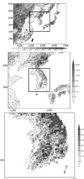
Fig. 1.

WRF domain and topography (shading, unit is m) for Domain 1 (upper panel, 27km spacing), Domain 2 (middle panel, 9km spacing), and Domain 3 (lower panel, 3km spacing). Shading indicates areas where the differences are statistically significant at the 90% confidence level.

Table 1.

The WRF physical schemes and references used in this study

Physics Schemes References

Microphysics WSM6 Lin

et al

. (1983)

Longwave RRTM Mlawer

et al

. (1997)

Shortwave Dudhia Dudhia (1989)

Land Surface Noah Chen and Dudhia (2001)

Planetary Boundary Layer YSU PBL Hong and Lim (2006)

Cumulus Kain-Fritsch Kain (2004)

(3)

이하

CGCM)

을 이용하여

CO

2가 배증된 장기 평형 기후를 생산하였다

.

^또한 ^한반도와 ^같이 ^{지리적으로}

복잡하고 좁은 지역의 기후를 모사하기 위하여

CGCM

^으로^생산된^대기^기후^자료를^경계^및^초기조

건으로사용하여역학적규모축소법으로

3km

까지 수 평 해상도를 높여

CO

2 배증에따른 한반도 상세 기 후를 생산하였다

.

모형이모사하는 한반도상세기후 예측 자료를토대로본연구에서는

CO

2배증에따른 농업기후지수변화를살펴보고자하였다

.

II. 모형 개요 및 실험 방법

2.1. 모형개요

본연구에서는지구를구성하는대기와해양

,

해빙

,

지면및생권의변화와이들간의 상호작용을고려하 는접합대순환모형을이용하여이산화탄소가배증된 기후를예측하였으며그결과를분석함으로써기후의 변화를살펴보았다

.

본연구에서사용한접합 대순환 모형은전지구장기기상예측과엘니뇨

/

라니냐의장기 예측을 위해 사용되어 예측성이 증명된

PNU CGCM(Pusan National University Coupled General Circulation Model)

^으로써

(Jeong and Ahn, 2007)

이 모형은 전구 규모의 대기 대순환 모형

NCAR/

CCM3(National Center for Atmospheric Research/

Community Climate Model Version3) AGCM (Atmo- spheric General Circulation Model)

과 전구 규모 해

양 대순환 모형인

MOM3(Modular Ocean Model

Version3) OGCM(Oceanic General Circulation Model), Ahn and Lee(2001)

^가 ^개발한^열역학

/

^역학 ^해빙^모형

으로 구성되어 있다

(Jeong and Ahn, 2007; Ahn and Hwang, 2005). CCM3

^의 ^수평 ^해상도는

T42(

^위경도

간격이 약

2.8125

^o인가우시안 격자

)

이다

.

연직층 개 수는

18

^층이며

,

^대기 ^최상층은

2.917hPa

^로 ^성층권을

포함한다

.

모형에 대한 더 자세한 설명은

Park and

Ahn(2004)

에제시되어있다

.

또한 전구규모의 접합대순환 모형으로부터 얻어진

결과를 바탕으로 한반도 영역

(Fig. 1)

에 대하여역학

적규모축소를실시하기위해서는중규모예보모형으 로 사용되는

WRF(Weather Research and Forecasting Version3, Skamarock

^{et al}

., 2008)

^를 ^{사용하였다}

. WRF

는완전압축

,

비정수계모형이다

.

연직좌표는지

형을 따르는정수계기압 좌표이며

Arakawa C

^격자

를사용한다

.

그리고고차수치계를사용하며

2

차와

3

차

Runge-Kutta

^시간 ^적분법을 ^포함한다

.

^이류항에

대해서는 수평과연직 방향 모두

2

차에서

6

차까지의 차분법을도입한다

.

^또한 ^플럭스^형태의^진단 ^방정식

을사용하여질량

,

운동량

,

엔트로피

,

스칼라양을보

존한다

.

이 실험에서 사용한 물리적방법은

Table 1

에제시하였으며

,

물리적방법은모든 도메인에대하 여동일하게적용하였다

. Fig. 1

은

WRF

의적분영역

을나타낸 그림으로영역

1(D01)

은동아시아 지역이

며

,

영역

2(D02)

는한반도전체를포함한지역이다

.

그

리고영역

3(D03)

^은^한반도^남한^지역으로^{설정하였다}

.

규모축소를위한

WRF

의

D01, D02, D03

의수평격자 간격

(

^개수

)

^은 ^각각

27(189

^×

152)km, 9(213

^×

201)km, 3(222

×

222)km

로써

Im

et al

.(2008(a), 2008(b))

의

20km

^간격의^격자보다^한층^조밀하다

.

^그리고^연직층

개수는

28

층이고대기최상층은

50hPa

이다

.

2.2. 실험방법

AGCM

의실험의 경우에는

1970

년

11

월부터

2005

년

10

^월까지

36

^년간^관측된^월평균^해수면^온도를^경

계 조건으로 두고

, NCEP/NCAR(National Centers for Environmental Prediction /National Center for Atmospheric Research)

재분석자료를초기조건으로 두었다

. 1979

년부터

2005

년까지 매해

9

월

1

일을 초 기조건으로 한 달 스핀업을 하여 매해

10

월

1

일 초 기장을생성하였다

. OGCM

의장기스핀업실험을위 하여

1979

년부터

1997

년까지

19

년평균된각월평균 관측 해수면온도를경계조건으로

AGCM

을먼저적

분하였다

.

^이 ^실험으로 ^생성된

AGCM

^{최하층에서의}

대기 상태 변수를

19

년간 월평균하여

OGCM

을적

분하기 위한 경계 자료를 생산하여

OGCM

^을

100

^년

간스핀업을하였다

.

그리고

AGCM

과동일한기간에

대하여

OGCM

^을 ^적분하여 ^매해

10

^월

1

^일 ^초기장을

생성하였다

.

구체적인 실험 방식은

Park and Ahn (2004)

을 따랐다

. CGCM

의 실험은 매해

10

월

1

일 초기장으로

1979

년부터

2005

년까지

27

년간

12

개월씩 적분하였다

.

이 때 매해 매달의

CO

2와

CH

4 농도는

CDIAC(Carbon Dioxide Information Analysis Center)

에서제공하는값을처방하여적분하였다

.

이러한 방법으로 생산된

2006

^년

10

^월

1

^일 ^초기장

을두가지의경우로나누어실험하였다

.

첫번째실 험

(1

^×

CO

2

)

^은^{표준실험으로써}

2006

^년

10

^월에^해당하는

(4)

CO

2농도

(376.7ppm)

를처방하고

,

두번째실험

(2

×

CO

2

)

은 배증실험으로써 두 배의

CO

2 농도

(753.4ppm)

를 처방하여 각각을

60

^년간 ^장기^{적분하였다}

.

^이^실험에

의해 산출된

1

시간 간격 자료를

WRF

의 초기 및경 계자료로사용하여매월

3

일전부터매월말일까지 적분을시행하였다

.

^이^때

,

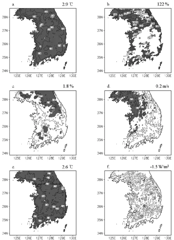
^지면의 ^수분과^온도는^접

Fig. 2.

Differences in climate variables (2

^×

CO

2

minus 1

^×

CO

2

) averaged from March to September for a. air temperature(

^o

C),

b. precipitation(%), c. relative humidity (%), d. wind speed(m/s), e. soil temperature(

^o

C), and f. solar radiation(W/m

²

).

(5)

합 모형의결과값을사용하였다

.

접합 모형의결과를

WRF

^의^{경계조건과}^{초기조건으로}^사용한^기간은

2057

년부터

2061

년까지

5

년동안의

3

월에서

9

월의자료이 다

.

^역학적^{규모축소법을}^위하여^둥지화

(nesting)

^방법

은 모든 영역에대하여피드백을 고려하여 좀더 신 뢰도 높은 결과를얻기 위해 양방향이둥지격자계를 적용하였다

.

III. 결 과

3.1. 기후변수의변화

Fig. 2

는

3

월에서부터

9

월까지의

D03

의 기상 및 토양 변수의

5

^년간

(2057-2061)

^평균 ^변화를 ^나타냈

으며

,

값은

2

×

CO

2와

1

×

CO

2차이로나타내었다

.

그리

고

10%

^유의 ^수준인^영역에^대하여^음영으로^나타내

었다

.

기온

(Fig. 2a)

의 변화를먼저 살펴보면

,

한반도 평균적으로

2.9

^o

C

상승을 보이며

,

이 값은

IPCC

AR4

에서 제시된

2080~2099

년 사이의 동아시아

(3.3

^o

C)

에서의 평균 온난화

(IPCC, 2007)

와 유사하다

.

지역적으로 서해안을 따라서기온 차이가가장 크게 나타나고 있다

.

강수

(Fig. 2b)

는평균적으로

1

×

CO

2일

때보다

22%

^정도^증가하는^것으로^보아^총^강수량은

1

×

CO

2와비슷한양을 모사하고 있으며

,

황해도지역 에강수가가장많이증가할것으로보인다

.

상대습도

(Fig. 2c)

는강원도 일대에서가장 큰차이를 보이며

,

전체적으로

1.8%

증가한것을 볼수있다

.

풍속

(Fig.

2d)

은큰 증감을보이지않으나

,

우리나라중서부 지

역에서다소 더증가한것을알수있으며

,

평균적으 로

0.2m/s

^증가를 ^나타낸다

.

^토양온도

(Fig. 2e)

^는 ^지

표면에서

1m

깊이까지의온도이다

.

대부분의지역에서 고르게 상승하는모습이며 평균값은

2.6

^o

C

^이다

.

^일사

량

(Fig. 2f)

은 다소 감소할 것으로 예상된다

.

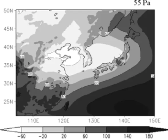
이러한 변화의원인분석위하여

D01

^에서의^{해면기압의}^변화

(Fig. 3)

를 제시하였다

.

이 값은

Fig. 2

와 동일한 기 간에 대하여

2

×

CO

2와

1

×

CO

2차이로나타내었다

.

한 반도 서쪽 주변에는해면기압의감소가있으며

,

동쪽 에서는 증가가 있을 것으로 나타난다

.

이로 인해

1

^×

CO

2일때보다

2

^×

CO

2일때

,

^황해도^지역에^저기압

이 발달하여 강수가증가할것이라는 것을 알수 있 다

.

^또한

,

^한반도^{평균적으로는}^{해면기압의}^차이가^거의

없을것으로보이는데

,

이것으로한반도평균강수량의 변화는큰차이가없을것이라는것을알수있다

.

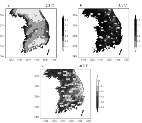
3.2. 최고기온및최저기온의변화

최고기온

(Fig. 4a)

은 동해안과 서해안에서 가장 큰

차이를보이며평균값은

2.8

^o

C

이다

.

최저기온

(Fig. 4b)

은평균적으로

3.1

^o

C

상승한것으로나타나며 서해안 지역에서가장 큰변화를보인다

.

최고기온보다최저 기온의상승폭이다소큰것으로나타나며이로인해 일교차는 약간 감소하는 것으로 모의되었다

.

한반도 평균적으로일교차

(Fig. 4c)

^는

0.2

^o

C

^의^감소를^보인다

.

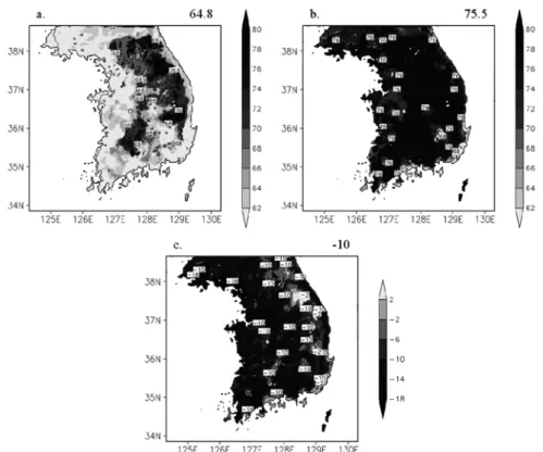
3.3. 봄철서리의변화

봄철서리는 밤시간동안의기온이

0

^o

C

이하일때 발생하는것으로정의하였으며

(Moonen

et al

., 2002), 3

월

~5

월의최저기온자료를이용하여분석하였다

. Fig.

5

는봄철

(3

월

~4

월

)

동안의평균서리일수의차이를나 타낸 것이며

, Ahn

^{et al}

.(2001)

^에서 ^제시한^방법으로

기상청관측소와

AWS

자료를이용하여오차를보정

한 값이다

.

^{오차보정은} ^절대적인 ^기준값을 ^이용하여

값을구하는농업지수에서만적용하였다

.

그리고분석 결과

5

월에는

1

×

CO

2와

2

×

CO

2모두서리일수가나타 나지않았기때문에그림에나타내지는않았다

.

먼저

,

서리일수는모든지역에서감소하였으며

,

증가한곳은 없었다

. 3

월

(Fig. 5a)

에는 한반도대부분지역에서서 리일수가

17

일정도감소할것으로보이며

,

특히내륙 지역에서큰 감소가발생할것으로예측된다

.

^그리고

봄철 평균적

(Fig. 4c)

으로 약

10

일 감소할것으로예

상된다

. Fig. 6

^은 ^봄철 ^{최저기온의}^차이를^나타낸^값

Fig. 3.

Differences in sea level pressure (Pa) for Domain 1

(2

×

CO

2

minus 1

×

CO

2

) averaged from March to September.

(6)

Fig. 4.

Differences in temperature (2

×

CO

2

minus 1

×

CO

2

) averaged from March to September for a. maximum temperature(

^o

C), b. minimum temperature(

^o

C) and c. diurnal temperature range(

^o

C).

Fig. 5.

Differences in frost days (2

×

CO

2

minus 1

×

CO

2

) for a. March(days), b. April(days) and c. averaged March to

April(days).

(7)

Fig. 6.

Differences in minimum temperature (2

^×

CO

²

minus 1

^×

CO

²

) in spring for a. March(

^o

C), b. April(

^o

C), and c. May(

^o

C).

Fig. 7.

Last frost date in spring for a. 2

×

CO

2

(days), b. 1

×

CO

2

(days), and c. 2

×

CO

2

minus 1

×

CO

2

.

(8)

으로

Fig. 4b

^와 ^비교해 ^보았을 ^때

,

^봄에 ^{최저기온의}

상승이더 크게발생할것으로예상된다

.

서리일수가 감소하는 반면에 봄철 최저기온은

3

^o

C

이상 증가할

것으로예상된다

. Fig. 7

은서리가마지막으로발생한

날짜를줄리안데이로나타낸것이며

,

서리일수와동일 한 방법으로관측을 이용하여오차를 보정한 값이다

. 2

×

CO

2는한반도평균적으로

64.8

일에 서리가마지막 으로발생하고

, 1

^×

CO

2는

75.5

^일에^{마지막으로}^서리가

발생하여

2

×

CO

2인 경우에 약

10

일 정도 빨리 서리 가종료될것으로보인다

.

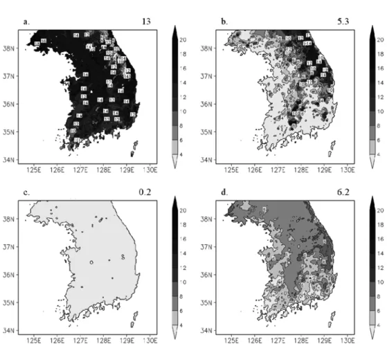
3.4. 식물온도의변화

식물기간은일평균기온이

5

^o

C

이상인일수를나타 내는지수로서영년생작물의재배관리에지표가되는 값이다

(Shim

^{et al}

., 2008). Fig. 8

^은 ^봄철 ^동안 ^일

평균기온이

5

^o

C

이상되는 일수의차이를 나타낸그 림이다

. 2

^×

CO

2일 때봄철 평균적으로

6.2

^일^정도 ^증

가하는것을알수있으며

, 3

월에가장 큰차이를보

인다

. Fig. 9

는 식물온도의 평균 출현초일의 차이를

나타낸그림으로

,

^{이산화탄소가}^배증된^기후에서^평균

Fig. 8.

Differences in days over 5

^o

C, 2

^×

CO

2

minus 1

^×

CO

2

in spring for a. March (days), b. April (days), c. May (days), and d. spring averaged (

^o

C).

Fig. 9.

Difference in first date of 5

^o

C in spring, 2

×

CO

2

minus 1

×

CO

2

.

(9)

식물온도의출현초일이

3.7

일정도빨라지는것을 알 수 있다

.

^그리고 ^한반도 ^{중부지역보다} ^{남부지역에서}

출현초일이앞당겨질것으로예상된다

.

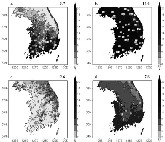
3.5. 작물온도의변화

과수재배에서중요시되는작물온도는일평균기온 이

10

^o

C

이상일 때를 가리키며

,

여름작물은 생육이 시작되고월동작물은발육이진행되는환경조건이된 다

(Shim

et al

., 2008). Fig. 10

은

3

월

, 4

월

, 5

월의 평균 일 평균기온이

10

℃ 이상인 날 수를

2

×

CO

2와

1

^×

CO

2차이로나타낸값이다

.

^{지역적으로}^남해안^지

역이동해안지역보다큰증가가있을것으로보이며

,

한반도 평균적으로

7.6

^일 ^증가하는^것을 ^알 ^수^있다

.

Fig. 11

은작물온도의평균출현초일의차이를나타낸

값으로평균적으로약

5.8

^일^빨라지는^것으로^예상되

며

,

강원도산맥지역에서는작물온도의출현초일이비 슷할것으로예상된다

.

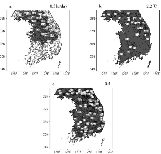
3.6. 기후생산력지수의변화

출수기부터출수기간

40

일간의평균기온

(Ta)

과일조 시간

(DS)

^으로 ^{기후생산력지수}

(Climatic Production

Fig. 10.

Differences in days over 10

^o

C (2

^×

CO

2

minus 1

^×

CO

2

) in spring. a. March (days) b. April (days), and c. May (days), and d. spring averaged (

^o

C).

Fig. 11.

Difference in first date of 10

^o

C in spring, 2

×

CO

2

minus 1

×

CO

2

.

(10)

(Shim

et al

., 2008).

CPI = DS(0.187-0.0034(Ta-22.7)

²

) (1)

10%

유의수준인영역에대하여음영으로나타내었

으며

,

^출수 ^후

40

^일^간의 ^평균 ^일조시간

(Fig. 12a)

^을

보면

,

한반도평균적으로

0.5 hr/40day

증가하는것을 알수있다

.

그리고지역적으로중북부

(

경기도와강원 도 내륙

)

지역에서

1 hr/day

이상 증가하고 그에 비 해 남해안 지역에서는

0.1 hr/40day

정도 감소하는 것으로보인다

.

평균 기온

(Fig. 12b)

는한반도평균적 으로 약

2.2

^o

C

정도 증가할 것으로보인다

.

그로 인 해기후생산력지수

(Fig. 12c)

^는^한반도^{평균적으로}

0.5

정도 증가하는 것을 알 수 있다

.

이 값은

Shim

et

al

. (2008)

^의 ^연구 ^분석에서^남해안 ^지역에서^약

1.0,

산간 고랭지

(

강원도

)

에서 약

0.6

의 값을 가지는것과 비교하면

,

상당한 증가라고 볼 수 있다

.

지역적으로 중북부지역에서남부지역보다큰증가가발생할것으 로예상된다

.

적 요

본연구에서는지구온난화에따른식물기간과작물 기간등과관련된농업기후지수의변화를살펴보기위

하여 접합 대순환 모형인

PNU CGCM

에 의해 모의

된

CO

2 배증 실험 결과를 지역기후 모형인

WRF

에

two-way double nesting

방법을이용하여역학적규모 축소법을 적용 후

,

그결과를 분석하였다

.

분석 기간 은 배증 실험 시작 후

51

^년부터

55

^년까지

5

^년 ^동안

Fig. 12.

Difference in a. duration of sunshine (hr), b. temperature (

^o

C), and c. climatic productivity index (2

^×

CO

2

minus 1

^×

CO

2

) for 40 days after heading date. Shading indicates areas where the differences are satistically significant at the 90%

confidence level.

(11)

의 3월~9월이다. 분석 결과 기온은 뚜렷하게 상승하는 모습을 볼 수 있었으며, 강수는 지역별로 차이를 보였 으나 전반적으로 증가할 것으로 예상되었다. 상대습도 와 토양온도도 증가하였으나 일사는 감소할 것으로 보 인다. 풍속은 지역별로 큰 차이 없이 다소 상승할 것 으로 모의되었다. 최저기온은 최고기온보다 상승폭이 커서 일교차는 줄어들 것으로 예상된다. 봄철 서리일 수는 감소하고, 마지막 서리일은 빨라질 것으로 나타 난다. 일 평균기온이 5 이상인 일수는 3월에 가장 큰 증가가 있을 것으로 보이며, 식물온도의 평균 출현초 일은 한반도 평균적으로 3.7일 정도 빨라지는 것을 알 수 있었다. 그리고 한반도 북부지역보다 남부지역에서 출현초일이 앞당겨질 것으로 예상된다. 일 평균 기온 이 10 이상 출현지속 기간인 작물온도의 평균 출현초 일은 평균적으로 17일 빨라질 것으로 보이며 지역적으 로 분석하였을 때, 강원도 산맥지역에서는 작물온도의 출현초일에 큰 변화가 없을 것으로 예상된다. 그리고 기후생산력 지수는 출수 후 40일간의 평균 일조시간과 기온의 상승으로 인해 증가할 것으로 예상된다. 따라 서 CO2 배증에 의해 변화된 한반도 기후는 식물 및 작물의 생장과 벼 생장에 좋은 영향을 미칠 것으로 예상된다. 따라서 지구 온난화에 따라 예상되는 한반 도 기후변화에 적합한 작부체계의 개선이 향후 필요할 것으로 생각된다. 그리고 본 연구는 하나의 시나리오 를 적용한 결과이므로 보다 다양한 시나리오를 적용하 여 그에 따른 농업기후지수 변화를 살펴보는 연구가 필요하다.

감사의 글

본 연구는 농촌진흥청 공동연구사업(과제번호:

200806A01036056과 200901OFT072454094)에 의해 수행되었습니다.

REFERENCES

Ahn, J. B., C. K. Park, and E. S. Im, 2001: Reproduction of regional scale surface air temperature by estimating systematic bias of mesoscale numerical model. Journal of the Korean Meteorological Society

38

(1), 69-80. (in Korean with English abstract)

Ahn, J. B., and J. A. Lee, 2001: Numerical study on the role of sea-ice using ocean general circulation model. The

Sea, Journal of the Korean Society of Oceanography

6

(4), 225-233. (in Korean with English abstract)

Ahn, J. B., and Y. J. Hwang, 2005: A study of predictability of CME/PNU CGCM for East Asia winter temperature.

Journal of the Korean Meteorological Society

41

(6), 943-954. (in Korean with English abstract)

Bonsal, B. R., X. Zhang, L. A. Vincent, and W. D. Hogg, 2001: Characteristics of daily and extreme temperatures over Canada. Journal of Climate

14

(9), 1959-1976.

Chen, F., and J. Dudhia, 2001: Coupling an advanced land- surface/ hydrology model with the Penn State/ NCAR MM5 modeling system. Part I: Model description and implementation. Monthly Weather Review

129

(4), 569- Dudhia, J., 1989: Numerical study of convection observed 585.

during the winter monsoon experiment using a mesoscale two-dimensional model. Journal of the Atmospheric Sciences

46

(20), 3077-3107.

Frich, P., L.V. Alexander, P. Della-Marta, B. Gleason, M.

Haylock, A.M.G. Klein Tank, and T. Peterson, 2002:

Observed coherent changes in climatic extremes during the second half of the twentieth century. Climate Research

19

, 193-212.

Heino, R., R. Brázdil, E. Førland, H. Tuomenvirta, H.

Alexandersson, M. Beniston, C. Pfister, M. Rebetez, G.

Rosenhagen, S. Rösner, and J. Wibig, 1999: Progress in the study of climate extremes in northern and central Europe. Climatic Change

42

(1), 151-181.

Hong, S. Y., and J. O. J. Lim, 2006: The WRF single- moment 6-class microphysics scheme (WSM6), Journal of the Korean Meteorological Society

42

(2), 129-151.

Im, E. S., J. B. Ahn, W. T. Kwon, and F. Giorgi, 2008:

Multi-decadal scenario simulation over Korea using a one-way double-nested regional climate model system.

Part 2: future climate projection (2021-2050). Climate Dynamics

30(

2/3), 239-254.

Im, E. S., J. B. Ahn, A. R. Remedio, and W. T. Kwon, 2008: Sensitivity of the regional climate of East/

Southeast Asia to convective parameterizations in the RegCM3 modelling system. Part 1: Focus on the Korean peninsula. International Journal of Climatology

28(

14), 1861-1877.

IPCC, 2007: Climate Change 2007: The Physical Science Basis. Contribution of Working Group I to the Fourth Assessment Report of the Intergovernmental Panel on Climate Change , Solomon, S., D. Qin, M. Manning, Z.

Chen, M. Marquis, K. B. Averyt, M. Tignor and H. L.

Miller (eds.), Cambridge University Press, Cambridge, United Kingdom.

Jeong, H. I., and J. B. Ahn, 2007: Long-term Predictability for El Nino/La Nina using PNU/CME CGCM. The Sea, Journal of the Korean Society of Oceanography

12(

3), 170-177. (in Korean with English abstract)

Kain, J. S., 2004: The Kain-Fritsch convective parameterization:

(12)

An update. Journal of Applied Meteorology

43

(1), 170- Lin, Y.-L., R. D. Farley, and H. D. Orville, 1983: Bulk 181.

parameterization of the snow field in a cloud model.

Journal of Applied Meteorology

22

(6), 1065-1092.

Meehl, G. A., C. Tebaldi, and D. Nychka, 2004: Changes in frost days in simulations of twentyfirst century climate.

Climate Dynamics

23

(5), 495-511.

Mlawer, E. J., S. J. Taubman, P. D. Brown, M. J. Iacono, and S.

A. Clough, 1997: Radiative transfer for inhomogeneous atmosphere: RRTM, a validated correlated-k model for the longwave. Journal of Geophysical Research Atmospheres

102

(D14), 16663-16682.

Moonen, A. C., L. Ercoli, M. Mariotti, A. Masoni, 2002:

Climate change in Italy indicated by agrometeorological indices over 122 years. Agricultural and Forest Meteorology

111

(1), 13-27.

Park H. S., and J. B. Ahn, 2004: Development of a new CGCM and ENSO hindcast experiment using the CGCM(I). Journal of the Korean Meteorological Society

40