1. Introduction
1)It is very difficult to estimate the sediment load from land surface because intensive-frequency sampling of the water is needed to quantify sediment loading during the rainy season.
The hydrologic model is a useful tool for estimating sedi- ment load, but it requires a significant amount of effort and professionals for the process, from model set-up to model calibration and validation. The Universal Soil Loss Equation (USLE) developed by the United States Department of Agriculture (Wischmeier and Smith, 1978), is widely used to estimate the amount of soil loss from watersheds because it is easy to apply and to evaluate the various best management
†To whom correspondence should be addressed.
This is an Open-Access article distributed under the terms of the Creative Commons Attribution Non-Commercial License (http://creativecommons.org/
licenses/by-nc/3.0) which permits unrestricted non-commercial use, distribution, and reproduction in any medium, provided the original work is properly cited.
practices to control soil loss. Various modified versions of USLE, such as the Modified USLE (MUSLE) (Williams and Berndt, 1977) and Revised USLE (RUSLE) (Renard et al., 1991), have been developed. The various versions of USLE have been linked with hydrologic models, such as GWLF, AGNPS, STORM, SWAT, and SWMM, to estimate sediment loads (U. S. EPA, 1997). Many researchers have further en- hanced USLE factors to allow more accurate estimates or easier use. Shabani et al. (2014) reported that the K factor is highly sensitive to the lime content in the soil and slope of the landscape, and proposed a new K value estimation meth- od considering the lime content and slope for a more accu- rate estimation. Auerswald et al. (2014) proposed a new equation to estimate the K factor, and Bagarello et al. (2013) developed a new expression to estimate the LS factor.
Zhang et al. (2011) proposed a method for estimating C and P factors using remote sensing technology. Park et al.
(2010) developed a SATEEC GIS system which can generate
Developing Suspended Sediment Delivery Ratio in the Lake Imha Watershed
Ji-Hong Jeon Donghyuk Choi Jae-Kwon Kim* Taedong Kim† Department of Environmental Engineering, Andong National University
*Environmental Management Corporation
임하호유역 유사유달공식 개발
전지홍․최동혁․김재권*․김태동† 안동대학교 환경공학과
*한국환경공단
(Received 12 October 2017, Revised 27 November 2017, Accepted 27 November 2017)
Abstract
The sediment delivery ratio (SDR) is widely used to estimate sediment loads by multiplying soil loss through the Revised Universal Equation (RUSLE). In this study, the SDR equation was developed for the Lake Imha watershed using soil loss calculated by RUSLE and sediment loads by the calibrated Hydrological Simulation. Program Fortran (HSPF). The ratio of watershed relief and channel length (Rf/Lch), the ratio of watershed relief and watershed length (Rf/Lb), curve number (CN), area (A), and channel slope (SLPch) demonstrated strong correlations with SDR. SDR equations were developed by a combination of subwatershed parameters by referring to the correlation analysis. The area based power functional SDR developed in this study showed significant errors at the point right after entering major tributaries, because SDR was unrealistically reduced when the watershed area increased significantly. The SLPch-based power functional SDR also showed extraordinary values when the channel slope was gradual. The SDR equation that showed the highest value of the coefficient of determination also presented unrealistic changes in the sediment loads within a relatively short river distance. The SDR equation SDR = 0.0003A0.198Rf⁄Lw1.167
was recommended for application to the Lake Imha watershed. Using this equation, sediment loads at the outlet of the Lake Imha watershed were calculated, and the HSPF parameters related to sediment in the uncalibrated subwatersheds were determined by referring to the sediment loads calculated with the SDR equation.
Key words : Calibration, HSPF, Lake Imha, Suspended sediment loads
daily time variant R and C factors.
Some fraction of eroded soil is lost by deposition in swales, on the flood plain, or in the channel itself. The mag- nitude of the loss of soil erosion within the drainage basin tends to increase with the drainage area (Walling, 1983).
Sediment delivery ratio (SDR) can be defined as the ratio of the erosion upslope of a point in the landscape to the sedi- ment delivered from that point (Kinnel, 2004), and can be expressed as:
SDR E
Y (1)
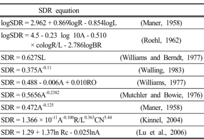
where Y is the amount of sediment yield delivered at some point, and E is the amount of eroded soil from the drainage area of the same point. Wade and Heady (1978) reported the sediment delivery ratio at the outlets of watersheds to range from 0.1 to 37.8% based on countrywide study of 105 agri- cultural production areas in the United States. Many re- searchers have proposed relationships between the sediment delivery ratio and watershed characteristics: basin relief, ba- sin length, drainage area, relief/length ratio, main channel slope, SCS curve number, and annual runoff. The SDR equations are shown in Table 1.
The differences in the equations cause different SDR values to be calculated for the same given drainage area, because SDR is strongly dependent on drainage heterogeneity includ- ing topography, climate, soil, vegetation cover, and land use condition, as well as their complex interactions (Lu et al., 2006). Although the model supports the SDR calculation tool, the user could be confused as to which SDR equation to select. The strength of the USLE series is that it is easy to find critical areas as a field scale and evaluate BMPs, but it has the weakness of potential error for estimating the sedi-
ment load due to inappropriate selection of the SDR equation.
As shown in ‘Part 1: HSPF calibration’, Hydrological Simulation. Program Fortran (HSPF) can estimate sediment loads relatively accurately, because hourly time step simu- lation can consider the rainfall intensity and provide a good representation of the high fluctuation of suspended sediment loads during high flow rates. However, determining the cali- bration parameter related to sediment simulation for un- calibrated subwatersheds is also an issue, because the default value does not represent the various conditions related to soil erosion.
In this study, an SDR equation was developed using SDRs of the six calibrated subwatersheds by implementing the ra- tio of soil loss of RUSLE and sediment loads of HSPF.
Using the new SDR equation, the sediment loads at an outlet of the Lake Imha watershed was calculated by multiplying SDR and soil loss of RUSLE, and a method is proposed for determining the uncalibrated HSPF parameters of ungauged subwatersheds using the sediment loads calculated by SDR and RUSLE.
2. Materials and Methods
2.1 RUSLE
The USLE was designed to estimate sheet and rill erosion from hillslope area, but not address soil deposition and chan- nel or gully erosion within a watershed (Renard et al., 1991). The RULSE is an index method containing factors that represent how climate, soil, topography, and land use af- fect rill and interrill soil erosion caused by raindrop impact and surface runoff. The RUSLE equation is as follows:
Loss RKLSCP (2)
where Loss is the soil loss(ton/ha·year), R is the rainfall ero- sivity factor, K is a soil erodibility factor, L is the slope length factor, S is the slope steepness factor, C is a cover management factor, and P is a supporting practices factor.
The R-factor represents the long-term average erosivity of the climate, calculated by the total rainfall energy (E) and the maximum 30 min rainfall intensity (I30) for rainfall events. The R-factor can be calculated as follows :
R N
∑i j EIi
(3)
E
i j
eiVi (4)
e exp (5)
where E is the total storm kinetic energy (MJ ha-1), I30 is the SDR equation
logSDR = 2.962 + 0.869logR - 0.854logL (Maner, 1958) logSDR = 4.5 - 0.23 log 10A - 0.510
× cologR/L - 2.786logBR (Roehl, 1962) SDR = 0.627SL (Williams and Berndt, 1977)
SDR = 0.375A-0.11 (Walling, 1983)
SDR = 0.488 - 0.006A + 0.010RO (Williams, 1977) SDR = 0.5656A-0.2382 (Mutchler and Bowie, 1976)
SDR = 0.472A-0.125 (Maner, 1958)
SDR = 1.366 × 10⁻¹¹A-0.100R/L0.363CN5.44 (Kinnel, 2004) SDR = 1.29 + 1.37ln Rc - 0.025lnA (Lu et al., 2006) where A is the drainage area, R is the basin relief, L is the basin length, BR is the bifurcation ratio, SLP is the slope of the main channel, RO is the annual runoff, and CN is the curve number.
Table 1. Proposed relationships between SDR and catchment characteristics
maximum 30-min intensity (mm h-1), N is number of years, ei is the rainfall energy per unit depth of rainfall (MJ ha-1 mm-1 h-1), I is the rainfall intensity (mm h-1), and ΔVi is the duration of the increment over which I is constant in hours (h). Guak calculated the R-factors in 2003 using equations (3) ~ (5) for eight rainfall gauge stations monitored every 1 minute within the Lake Imha watersheds (Fig. 1 and Table 2) (Guak, 2007). A grid-based R-factor map was generated using the Spline interpolation method of ArcView 3.0 (ESRI, 2002), as shown in Fig. 2.
The K-factor was determined using the Erickson triangular nomograph method, considering the percentage of sand, silt, and clay in the soil (Erickson, 1997). A 1:2500 scaled soil map including information on soil texture was obtained from the Korean National Academy of Agricultural Science.
K-values were allocated to the soil map and a grid-based K-factor map was generated, as shown in Fig. 2.
A grid-based LS-factor map was generated using the SATEEC GIS system (Park et al., 2010) with the Digital Elevation Model (DEM) obtained from the Environmental Geographic System (EGIS) (ME, 2014). The SATEEC GIS
system uses Moore and Burch’s method, using the following equation (Moore and Burch, 1986):
LS
A
sinθ
(6)where A is the flow accumulation cell size, and q is the slope angle in degrees.
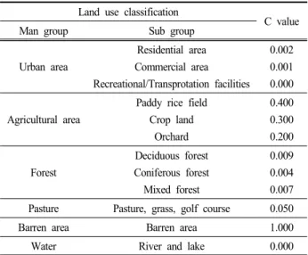
Park (2003) allocated C values to land use as classified by the Korean Ministry of Environment by referencing docu- ments, for which the C values are shown in Table 3. The land use classification map was obtained from EGIS, and the grid-based C-factor map is shown in Fig. 2.
The P-factor considers the support practice of protecting cultivated areas from soil erosion. Williams and Smith pro- posed P values considering a combination of land slope and the supporting cropland practices including contouring, con- tour strip cropping, and terracing (Wischmeier and Smith, 1978). In Korea, rice paddy fields and other agricultural areas can be considered as terrace systems and contour till- age, respectively (Guak, 2007; Park, 2003). The P values, from Williams and Smith (Wischmeier and Smith, 1978), are shown in Table 4. The p-factor map was generated using DEM and land use map and is shown in Fig. 2.
Station R factor Station R factor
Cheongsong 46.24 Seokbo 308.92
Budong 188.42 Yeongyang 67.55
Bunam 112.00 Subi 281.83
Jinbo 78.85 Ilwol 176.85
Fig. 1. Study area.
Table 2. R-values from 2003 data for eight rainfall gauge stations within the Lake Imha watershed
Land use classification
C value
Man group Sub group
Urban area
Residential area 0.002
Commercial area 0.001
Recreational/Transprotation facilities 0.000
Agricultural area
Paddy rice field 0.400
Crop land 0.300
Orchard 0.200
Forest
Deciduous forest 0.009 Coniferous forest 0.004
Mixed forest 0.007
Pasture Pasture, grass, golf course 0.050
Barren area Barren area 1.000
Water River and lake 0.000
Table 3. C-values for land use classification
Slope (%) Contouring Terracing
1 ~ 2 0.60 0.12
3 ~ 12 0.55 0.11
13 ~ 20 0.75 0.10
20 ~ 25 0.90 0.18
over 25 1.00 0.20
Table 4. P-values for the combination of land slope and supporting cropland practices.
2.2 Research approaches
The SATEEC GIS system was used to generate the annual soil loss map for 2003. The significant water quality prob- lem, especially high turbidity concentration by soil loss, in the Imha multi-purpose dam occurred in 2003. An overview of the application of the SATEEC GIS system is shown in Fig. 3 (Lim et al., 2005). Total suspended sediment load at the outlet of subwatershed simulated by HSPF was consid- ered as the suspended sediment loads because HSPF consid- ers the deposition or scour in streams. The research was div-
ided by part 1 which was performed by Jeon et al. (2016) and part 2. This paper concerns part 2. A diagram of the modeling approach is shown in Fig. 5.
In Part 1, HSPF was calibrated at the uncalibrated sub- watersheds (Fig. 1) by matching with sediment loads at the outlet of the Lake Imha watershed, which were calculated by soil loss and SDR. The process of validation was not per- formed due to the data limitation. The soil loss was clipped for the subwatersheds and the suspended sediment loads from subwatersheds 4, 9, 13, 15, 36, and 46 was calculated Fig. 2. The 30×30 m grid based RUSLE factor maps for the Lake Imha watershed.
by HSPF (Fig. 1).
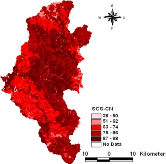
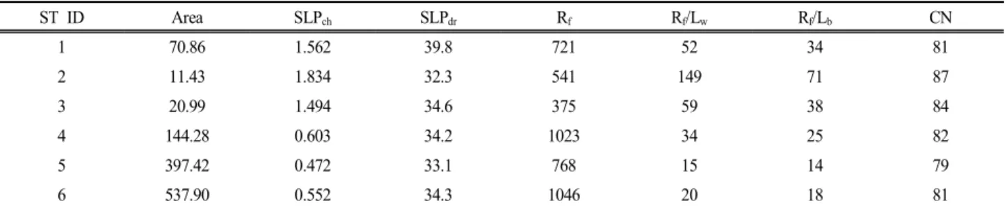
In Part 2, SDRs of the six calibrated subwatersheds for 2003 were calculated using the ratio of soil erosion by RUSLE and suspended sediment loads with the calibrated HSPF. Various topographic parameters were used in devel- opment of the SDR equations with reference to Table 1. The parameters included area (A, km2), watershed relief (Rf, m), curve number (CN), channel slope (SLPch), drainage slope (SLPdr), the ratio of watershed relief to watershed length (Rf/Lb, m/km), and the ratio of watershed relief to main channel length (Rf/Lw, m/km). Jeon et al. (2016) optimized the curve number for the combination of land use and hy- drologic soil group for the Lake Imha watershed. The cali- brated grid based on the CN map by Jeon et al. was used in this study (Fig. 4). The watershed relief was calculated by taking the difference between the highest and lowest ele- vations using DEM. Channel and drainage slope were calcu- lated using the BASINS Delineation Tool. The SDR equa- tions developed in this study were evaluated by comparing
the magnitude of the change in sediment loads within the subwatershed. Statistical analyses were performed with the IBM SPSS Statistics program (ver.21). Sediment loads at the outlet of the Lake Imha watershed were calculated by multi- plying soil erosion calculated with RUSLE and the SDR cal- culated using the SDR equation.
3. Results and Discussion
3.1 Development of SDR equation
The application of RUSLE revealed that about 2,070,580 ton/year of soil eroded from Lake Imha watershed during 2003. The LS-factor and soil erosion maps obtained using the SATEEC GIS system are shown in Figs. 6 and 7. The SATEEC GIS system is a useful tool for the application of RUSLE and analysis of the spatial distribution of soil erosion. The SDRs calculated by the ratio of soil loss from Fig. 3. Diagram of SATEEC GIS system application.
Fig. 4. SCS-CN map of the Lake Imha watershed.
Fig. 5. Flow diagram of research approaches.
ST ID Sub- watershed
Soil loss (ton/yr)
Area (ha)
Sediment
loads SDR
1 4 7,086 7,086 9,810 0.078
2 9 1,143 1,143 7,410 0.172
3 13 2,099 2,099 1,160 0.042
4 15 14,428 14,428 10,982 0.052
5 36 39,742 39,742 7,730 0.025
6 46 53,790 53,790 35,100 0.045
Table 5. Calculated SDRs using soil loss by RUSLE and sediment loads by HSPF
RUSLE and sediment load from HSPF for the calibrated subwatersheds are presented in Table 5. The SDRs ranged from 0.025 to 0.172, and decreased with increasing drainage area. The subwatershed parameters and correlation analysis with the SDRs are shown in Tables 6 and 7, respectively.
SDRs were strongly correlated with the Rf/Lw, Rf/Lw, CN, and SLPch, showing correlation coefficients (R) of 0.95, 0.93, 0.80, and 0.76, respectively. The SDR equations for the Lake Imha watershed were developed, as shown in equations
(7) ~ (11), referring to Table 1 and the results of the correla- tion analysis.
SDR A R (7)
SDR SLPch R (8)
SDR RfLw R (9)
SDR ARfLwR (10) Fig. 6. LS and soil loss map within the Lake Imha watershed using the SATEEC GIS system.
Fig. 7. Soil loss maps for the subwatersheds covered by monitoring gauge stations.
SDR ARfLwCN R (11) Some SDRs calculated by equation (8) were about zero when the channel slope was gradual, as shown in Fig. 8, in- dicating that equation (8) was not appropriate for use as the SDR equation for the Lake Imha watershed. The differences of sediment inflow and outflow at outlet 33 calculated with equations (7) and (11) were significant, showing differences of -48% and 28%, respectively (Table 8). Considering the relatively small area of subwatershed 33 (14.8 km2), those differences seem unrealistic. At the point of outlet 33 and
47, equations (9) and (10) generated similar SDRs and were reasonable compared with (7) and (11) so the two equations could be recommended for SDR equation in the Lake Imha watershed.
Many researchers have proposed area-based power func-
ST ID Area SLPch SLPdr Rf Rf/Lw Rf/Lb CN
1 70.86 1.562 39.8 721 52 34 81
2 11.43 1.834 32.3 541 149 71 87
3 20.99 1.494 34.6 375 59 38 84
4 144.28 0.603 34.2 1023 34 25 82
5 397.42 0.472 33.1 768 15 14 79
6 537.90 0.552 34.3 1046 20 18 81
Table 6. Characteristics parameters of six calibrated subwatersheds as determined by HSPF
SDR Area Rf CN SLPch SLPdr Rf/Lb Rf/Lw
SDR 1.00 -0.52 -0.39 0.80 0.76 -0.14 0.93** 0.95**
Area -0.52 1.00
Rf -0.39 0.69 1.00
CN 0.80 -0.68 -0.57 1.00
SLPch 0.76 -0.83* -0.78 0.76 1.00
SLPdr -0.14 -0.22 0.03 -0.33 0.26 1.00
Rf/Lb 0.93** -0.73 -0.62 0.94** 0.87* -0.17 1.00
Rf/Lw 0.95** -0.68 -0.58 0.92 0.83* -0.23 0.995** 1.00
Note: * significant at the 0.01 level (2-tailed)
** significant at the 0.05 level (2-tailed)
Table 7. Correlation analysis between SDR and the catchment parameters
Fig. 8. Comparison of the SDRs for six calibrated sub- watersheds calculated by HSPF and RUSLE through the SDR equations.
Fig. 9. Sediment mass balance between subwatersheds 33 and 47.
tional SDR equations that decrease with increasing drainage area (Table 1). However, this type of equation can sometimes have significant error at watersheds that have major tribu- taries close to the outlet, as is the case for the Lake Imha watershed. The area-based power functional SDR equation in this study would be unrealistically decreased after entering major tributaries that have relatively large drainage areas.
3.2 HSPF calibration for uncalibrated subwatersheds HSPF was calibrated for uncalibrated subwatersheds using the sediment load calculated by multiplying the soil loss and SDR using equation (10), named the ‘SDR equation’ in Table 9, instead of the observed sediment load. Table 6 shows the sediment loads of Lake Imha by calibrated HSPF (HSPFcal), by using the calibrated HSPF parameters of the spatial nearest neighbor (HSPFemp), and by using the default HSPF parameters (HSPFdef). The relative errors were calcu- lated by the difference between the SDR equation and the three kinds of HSPF simulation results. Although the un- calibrated subwatershed area was 37% of the total Lake Imha watershed, HSPFdef and HSPFemp caused significant er- rors, showing 112% and 48% of relative errors, respectively.
A more reasonable method for the determination of HSPF parameters related to sediment calibration was to use the sediment load determined by RUSLE with the SDR equation. U. S. EPA (2006) guided the sediment calibration of HSPF, and proposed calibration of HSPF coupled with RUSLE and SDR. However, the SDR equation is very sensi- tive to site specifications, so the user should carefully select an accurate SDR equation for use.
3.3 Characteristics of suspended sediment inflow to Lake Imha
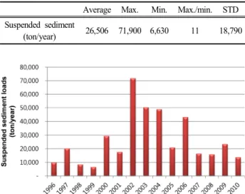
The simulated yearly suspended sediment inflow to Lake
Imha during 1996 ~ 2010, calculated by HSPF, and the statistical analysis are shown in Fig. 10 and Table 10, respectively. The average yearly suspended sediment inflow to Lake Imha was 26,506 ton/year. A significantly higher in- flow of suspended sediment to Lake Imha occurred during 2002, 71,900 ton/year. The maximum yearly suspended sedi- ment load was 11 times higher than the minimum loads.
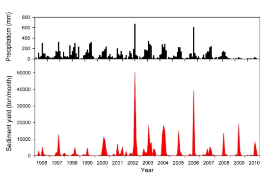
Statistical analysis of the monthly suspended sediment loads entering Lake Imha calculated by HSPF for 1996 ~ 2000 is shown in Table 11 and Fig. 11. The highest monthly suspended sediment was loaded during July, showing 12,627 ton/month, which was up to 40% of the total yearly load.
The second and third highest loads were 7,369 ton/month (28%) during August and 2,996 ton/month (11%) during June. Most of the suspended sediment entering Lake Imha was loaded during June ~ August, amounting to 79% of the
Average Max. Min. Max./min. STD Suspended sediment
(ton/year) 26,506 71,900 6,630 11 18,790 Table 10. Statistical analysis of the yearly suspended sedi-
ment loads entering Lake Imha for 1996 ~ 2010
Site Sediment loads Relative error
SDR equation* HSPFcal HSPFemp HSPFdef HSPFcal HSPFemp HSPFdef
Lake Imha watershed 43,706 50500 69100 98700. 8% 48% 112%
Note: * Equation (10) in Table 9
Table 9. Comparison of the sediment load at the outlet of the Lake Imha watershed calculated by HSPF calibration coupled with RUSLE employing calibrated parameters of the nearest monitoring station and by default parameters
Equation Subwatershed 33 Subwatershed 47 Difference between
33 ~ 47
Inflow Outflow SDR Difference Outflow SDR
7 35638 24075 0.013 -48% 27743 0.013 13%
9 48384 44478 0.024 -9% 39,715 0.019 -12%
10 50011 52527 0.028 5% 43706 0.021 -20%
11 53175 73914 0.040 28% 48491 0.023 -52%
Table 8. Inflow and outflow of suspended sediment between subwatersheds 33 and 47
Fig. 10. Yearly suspended sediment inflow to Lake Imha during 2000 ~ 2010.
total yearly sediment load. This is a common characteristic of runoff and nonpoint source pollution loaded in the Asian summer monsoon climate, for which most rainfall events oc- cur during June ~ August (Kettering et al., 2012; Kim et al., 2014).
4. Conclusions
In this study, SDRs were calculated using the ratio of the soil loss by RUSLE and the sediment loads by the HSPF simulation at six calibrated subwatersheds within the Lake Imha watershed, and an SDR equation for application to the Lake Imha watershed was developed. The correlation analy- sis indicated that the ratio of watershed relief to main chan-
nel length (Rf/Lch), the ratio of watershed relief to watershed length (Rf/Lw), curve number (CN), and area (A) showed strong correlations with SDR. As a result of SDR equation development, the channel slope-based SDR equation calcu- lated SDR as 0.0 when the channel slope was gradual. The SDR equation including Rf/Lch alone or Rf/Lch and A as in- dependent variables was recommended for application to the Lake Imha watershed. The SDR equation is empirical and influenced greatly by geomorphological characteristics of catchment or river. The documented SDR equation devel- oped from another site could generate potential error in esti- mating the delivered suspended sediment loads. Default HSPF parameters employed or the spatial nearest neighbor for uncalibrated subwatersheds demonstrated potential errors, showing 112% and 48% relative errors, respectively, com- pared with the sediment load calculated by multiplying the soil loss by RUSLE and the SDR calculated with the equation. The HSPF parameters of the uncalibrated sub- watersheds covering 37% of the Lake Imha watershed area were determined by matching with the sediment load. The SDR equation developed in this study is empirical model that can be applied on to the Lake Imha watershed and has potential errors when applied to other watershed. To de- termining the HSPF parameters at ungauged watersheds, the sediment load calculated by RUSLE and use of the SDR equation developed in the watershed is recommended.
Acknowledgments
This work was supported by a grant from 2015 Research Funds of Andong National University.
Month Average Max. Min. STD
Jan. 181 2,610 0 672
Feb. 50 319 0 96
Mar. 676 4,110 0 1,219
Apr. 328 1,970 4 555
May 628 2,060 7 694
Jun. 2,996 13,400 1 3,668
Jul 10,546 39,400 17 10,911
Aug. 7,396 50,500 207 12,627
Sep. 2,421 9,940 14 3,068
Oct. 442 5,140 0 1,320
Nov. 494 4,190 0 1,077
Dec. 347 3,460 0 937
Table 11. Statistical analysis of monthly suspended sedi- ment loads entering Lake Imha for 1996 ~ 2010
Fig. 11. Monthly suspended sediment inflow to Lake Imha during 1996 ~ 2010.
References
Auerswald, K., Fiener, P., Martin, W., and Elhaus, D. (2014).
Use and Misuse of the K Factor Equation in Soil Erosion Modeling: An Alternative Equation for Determining USLE Nomograph Soil Erodibility Values, CATENA, 118, 220-225.
Bagarello, V., Ferro, V., and Pampalone, V. (2013). A New Expression of the Slope Length Factor to Apply USLE-MM at Sparacia Experimental Area (Southern Italy). CATENA, 102, 21-26.
Environmental Systems Research Institute (ESRI). (2002).
What’s New in ArcView 3.1, 3.2, and 3.3, ESRI: Redlands, CA, USA.
Erickson, A. J. (1997). Aids for Estimating Soil Erodibility – K Value Class and Soil Loss Tolerance, USDA-SCS, Salt Lake City, Utah, USA.
Guak, D. W. (2007). Selection of Soil Erosion Source Area of Dam-basins Using GIS, Master thesis, Chonbuk National University, Chonbuk, Korea . [Korean Literature]
Jeon, J. H., Park, C. G., Choi, D., and Kim, T. (2016).
Characteristics of Suspended Sediment Loading Under Asian Summer Monsoon Climate Using the Hydrological Simulation Program-FORTRAN, Water, 9(1), 44.
Kettering, J., Park, J. H., Lindner, S., Lee, B., Tenhunen, J., and Kuzyakov, Y. (2012). N Fluxes in an Agricultural Catchment Under Monsoon Climate: A Budget Approach at Different Scales, Agriculture, Ecosystems & Environment, 161, 101-111.
Kim, Y. J., Kim, H. D., and Jeon, J. H. (2014). Characteristics of Water Budget Components in Paddy Rice Field under the Asian Monsoon Climate: Application of HSPF-Paddy Model, Water, 6, 2041-2055.
Kinnel, P. I. A. (2004). Sediment Delivery Ratios: A Misaligned Approach to Determining Sediment Delivery from Hillslopes, Hydrological Porcesses, 18, 3191-3194.
Lim, K. J., Sagong, M., Engel, B. A., Tang, Z., Choi, J., and Kim, K. S. (2005). GIS-based Sediment Assessment Tool, CATENA, 64, 61-80.
Lu, H., Moran, C. J., and Prosser, I. P. (2006). Modelling Sediment Delivery Ratio Over the Murray Darling Basin, Environmental Modelling & Software, 21, 1297-1308.
Maner, S. B. (1958). Factors Influencing Sediment Delivery Raties in the Red Hills Physiographic Area, Transactions American Geophysical Union, 39, 669-675.
Minstry of Environment (ME). (2014). Environmental Geographic Information Service (EGIS), http://egis.me.go.kr/ (accessed 24 Jun. 2014).
Moore, I. and Burch, G. (1986). Physical Basis of the Length-slope Factor in the Universal Soil Loss Equation, Soil Science Society of America Journal, 50, 1294-1298.
Mutchler, C. K. and Bowie, A. J. (1976). Effect of Land Use on Sediment Delivery Ratios, In: Proceedings of the Tird
Federal Inter-Agency Sedimentation Conference, U.S. Water Resources Council, Washington, D.C., 1-11-1-12.
Park, K. H. (2003). Soil Erosion Risk Assessment of the Geumho River Watershed Using GIS and RUSLE Methods, Journal of the Korean Association of Geographic Information Studies, 6, 24-36. [Korean Literature]
Park, Y. S., Kim, J., Kim, N. W., Kim, S. J., Jeon, J. H., Engel, B. A., Jang, W., and Lim, K. J. (2010). Development of New R, C and SDR Modules for the SATEEC GIS System, Computers & Geosciences, 36, 726-734.
Renard, K. G., Foster, G. R., Weesies, G. A., and Porter, J. P.
(1991). RUSLE: Revised Universal Soil Loss Equation, Journal of Soil and Water Conservation, 6, 30-33.
Roehl, J. E. (1962). Sediment Source Areas, Delivery Ratios and Influencing Morphological Factors, International Association of Scientific Hydrology, 59, 202-213.
Shabani, F., Kumar, L., and Esmaeili, A. (2014). Improvement to the Prediction of the USLE K Factor, Geomorphology, 204, 229-234.
Spaeth Jr, K. E., Pierson Jr, F. B., Weltz, M. A., and Blackburn, W. H. (2003). Evaluation of USLE and RUSLE estimated soil loss on rangeland, Journal of Range Management, 234- 246.
United States Environmental Protection Agency (U. S. EPA).
(1997). Compendium of Tool for Watershed Assessment and TMDL Development, EAP841-B-97-006, Office of Water (4503F), United States Environmental Protection Agency, Washington DC, USA.
United States Environmental Protection Agency (U. S. EPA).
(2006). BASINS Technical Note 8 - Sediment Parameter and Calibration Guidance for HSPF, Office of Water 4305, Washington DC, USA.
Wade, J. C. and Heady, E. O. (1978). Measurement of Sediment Control Impacts on Agriculture, Water Resources Research, 14, 1-8.
Walling, D. W. (1983). The Sediment Delivery Problem, Journal Hydrology, 65, 209-237.
Williams, J. R. and Berndt, H. D. (1977). Sediment Load Computed with Universal Equation, Journal of the Hydraulics Division, 98, 2087-2098.
Williams, J. R. (1977). Sediment Delivery Ratios Determined with Sediment and Runoff Models, AIHS-AISH publication, 122, 168-179.
Wischmeier, W. H. and Smith, D. D. (1978). Predicting Rainfall Erosion Losses, USDA Agricultural Research Service Handbook 537, USDA, Washington DC, USA.
Zhang, W., Zhang, Z., Liu, F., Qiao, Z., and Hu, S. (2011).
Estimation of the USLE Cover and Management Factor C Using Satellite Remote Sensing: A Review, Geoinformatics, 19th International Conference on, 1-5, Shanghai, China.