Bayesian Test for the Difference of Exponential Guarantee Time Parameters

2005, Vol. 16, No. 4, pp. 1095∼1106

Bayesian Test for the Difference of Exponential Guarantee Time Parameters

Sang Gil Kang¹⁾ ⋅ Dal Ho Kim²⁾ ⋅ Woo Dong Lee³⁾

Abstract

When X and Y have independent two parameter exponential distributions, we develop a Bayesian testing procedures for the equality of two location parameters. The reference prior in non-regular exponential model is derived. Under this reference prior, we propose a Bayesian test procedures for the equality of two location parameters using fractional Bayes factor and intrinsic Bayes factor. Simulation study and some real data examples are provided.

Keywords : Exponential Location Parameter, Fractional Bayes Factor, Intrinsic Bayes Factor, Reference Prior

1. INTRODUCTION

The two parameter exponential distribution plays an important role in the field of life testing and reliability theory since it is the only continuous distribution with a constant hazard function. The reciprocal of the scale parameter is the hazard rate. The location (threshold) parameter can translate the distribution along the time axis, so it is also known as the minimum life or guarantee time parameter. The guarantee time parameter can be used to model warranty periods for some products.

The present paper focuses on Bayesian testing procedure for the equality of two location parameters. In Bayesian testing problem, the Bayes factor under proper 1) First Author : Department of Applied Statistics, Sangji University, Wonju, 220-712,

Korea

E-mail : [email protected]

2) Department of Statistics, Kyungpook National University, Taegu, 702-701, Korea

3) Corresponding Author : Department of Asset Management, Daegu Hanny University, Kyungsan, 712-715, Korea

E-mail : [email protected]

priors or informative priors have been very successful. However, limited information and time constraints often require the use of noninformative priors.

Since noninformative priors such as Jeffreys' priors or reference priors (Berger and Bernardo, 1989, 1992) are typically improper so that such priors are only defined up to arbitrary constants which affects the values of Bayes factors.

Spiegalhalter and Smith (1982), O'Hagan (1995) and Berger and Pericchi (1996) have made efforts to compensate for that arbitrariness.

Berger and Pericchi (1996) introduced the intrinsic Bayes factor using a data-splitting idea, which would eliminate the arbitrariness of improper priors.

O'Hagan (1995) proposed the fractional Bayes factor. To remove the arbitrariness in Bayes factor, he used to a portion of the likelihood with a so-called the fraction b (See Sang Gil Kang and Hee Chun Lee (2004)). These two approaches mentioned above have shown to be quite useful in many statistical areas.

For the statistical inference of the exponential distribution, Epstein and Tsao (1953) studied some statistical tests for two exponential distributions. Epstein and Sobel (1954) obtained the minimum variance unbiased estimator for the scale and location parameters. The shrinkage estimators for the scale parameter have been proposed by Bhattacharya and Srivastava (1974). Chiou and Han (1989) proposed a pre-test estimator and a pre-test shrinkage estimator for the location parameter.

Chiou and Miao (2004) studied the shrinkage estimator for the difference between location parameters.

Almost all the work mentioned above is the analysis based on the classical point of view, there is a little work on this problem from the viewpoint of the objective Bayesian framework. Because the two parameter exponential distribution is the non-regular case, so the noninformative priors such as reference prior or probability matching prior were hard to derive. Since almost all the theory related to these priors were developed based on the assumption of regular distribution.

Recently, Ghosal (1997, 1999) developed the procedures to derive the reference and matching priors for non-regular cases. Using his results, we feel a strong necessity to develop objective Bayesian testing procedure for the difference between location parameters. For dealing this problem, we use the fractional Bayes factor (O'Hagan, 1995) and the intrinsic Bayes factor (Berger and Pericchi, 1996).

The outline of the remaining sections is as follows. In Section 2, using the reference priors, we provide the Bayesian testing procedure based on the fractional Bayes factor and intrinsic Bayes factor for the testing equality of two location parameters. In Section 3, simulation study and some real examples are given.

Section 4 devotes some conclusions of our Bayesian test procedure.

2. BAYESIAN TEST PROCEDURES

2.1 Preliminaries

Models (or Hypotheses) H₁, H₂, …, H_q are under consideration, with the data x = ( x₁,x₂, … ,x_n) having probability density function f_i( x ∣ θ_i) under model H_i,i= 1,2,…,q. The parameter vectors θ_i are unknown. Let π_i( θ_i) be the prior distribution of model Hi, and let pi be the prior probabilities of model Hi,

i = 1,2,…,q. Then the posterior probability that the model H_i is true is

P( H_i∣ x ) =

(

)

B_ji= m_j( x ) m_i( x ) =

⌠⌡f^j( x ∣ θ_j)π_j( θ_j)d θ_j

⌠⌡fⁱ( x∣ θ_i)π_i( θ_i)d θ_i . (2)

The Bji interpreted as the comparative support of the data for the model j to i. The computation of B_ji needs specification of the prior distribution π_i( θ_i) and π_j( θ). Usually, one can use the noninformative prior, often improper, such as uniform prior, Jeffreys prior, reference prior or probability matching prior. Denote it as π^N_i. The use of improper priors π^N_i(⋅) in (2) causes the B_ji to contain unspecified constants. To solve this problem, O'Hagan (1995) proposed the fractional Bayes factor for Bayesian testing and model selection problem as follow.

When the π^N_i( θ_i) is noninformative prior under H_i, equation (2) becomes

B^N_ji=

⌠⌡f^j( x ∣ θ_j)π^N_j( θ_j)d θ_j

⌠⌡fⁱ( x∣ θ_i)π^N_i( θ_i)d θ_i .

Then the fractional Bayes factor of model Hj versus model Hi is

B^F_ji= B^N_ji⋅

⌠⌡f^bi( x ∣ θ_i)π^N_i( θ_i)d θ_i

⌠⌡f^bj( x∣ θ_j)π^N_j( θ_j)d θ_j ,

and f_i( x ∣ θ_i) is the likelihood function and b specifies a fraction of the likelihood which is to be used as a prior density. He proposed three ways for the choice of the fraction b. One frequently suggested choice is b = m/n, where m is the size of the minimal training sample, assuming this is well defined. (see O'Hagan, 1995, 1997 and the discussion by Berger and Mortera of O'Hagan, 1995).

Berger and Pericchi (1996) proposed the intrinsic Bayes factor (IBF) for Bayesian testing and model selection. The arithmetic intrinsic Bayes factor is given by

B^I_ji= B^N_ji⋅ 1 L ∑^L

l = 1B^N_ij( x( l )), where

B^N_ij( x( l)) = m_i( x( l)) m_j( x( l)) =

⌠⌡fⁱ( x( l) ∣ θ_i)π^N_i( θ_i)d θ_i

⌠⌡f^j( x( l)∣ θ_j)π^N_j( θ_j)d θ_j .

Here x( l) is minimal training sample and L is the number of all possible minimal training samples.

2.2 Bayesian Test

Let X be a two parameter exponential distribution with density function

f(x∣η, θ) = 1

θ exp { - x- η

θ }, x > η, θ > 0, (3) where η is the location parameter (guarantee parameter) and θ is the scale parameter. Suppose that X = ( X₁,…,X_n1) is a random sample of size n₁ from a two parameter exponential distribution with location parameter η₁ and scale parameter θ1 and Y = ( Y₁,…,Y_n2) is a random sample of size n₂ from a two parameter exponential distribution with location parameter η₂ and scale parameter

θ₂. Then the joint probability density function is

f( x, y ∣η₁,η₂,θ₁,θ₂) = θ^{- n}₁ ¹θ^{- n}₂ ²exp { - n₁( x- η₁)

θ₁ - n₂( y- η₂) θ₂ }, where θ1> 0, θ₂> 0, x_i> η₁, i = 1, …, n₁ and yj> η₂, j = 1, …, n₂, and x and y are the sample mean for each population.

We want to test the hypotheses H1:η₁= η₂ vs. H2:η₁≠η₂. Our interest is to develop a Bayesian test based on the fractional and intrinsic Bayes factors for H1

vs. H₂ under the noninformative priors. The two parameter exponential distribution is belong to non-regular cases. But for non-regular cases, the reference is developed by Ghosal (1997). In our model (3), the reference prior is given by π( η,θ) ∝ 1/θ. For details, see Appendix 1.

2.2.1 Bayesian Test using the Fractional Bayes Factor

Under the hypothesis H1, the reference prior for η( ≡η1= η₂), θ₁ and θ2 is π₁(η,θ₁,θ₂) = θ₁^{- 1}θ₂^{- 1}.

The derivation of the reference prior for η, θ₁ and θ₂, and the propriety of the posterior distribution under this reference prior are given in Appendix 1.

The likelihood function under H₁ is

L( η, θ₁,θ₂∣ x, y ) = θ^{- n}₁ ¹θ^{- n}₂ ²exp { - n₁( x- η)

θ₁ - n₂( y- η)

θ₂ }

Then the element of fractional Bayes factor under H1 is given by

m^b₁( x, y) = ⌠⌡

mx, y

0

⌠⌡

∞ 0

⌠⌡

∞

0 L^b(η,θ₁,θ₂∣ x, y )π₁(η,θ₁,θ₂)dθ₁dθ₂dη = ( n₁b )^{− n1b}( n₂b )^{− n2b}Γ ( n₁b ) Γ ( n₂b )

: 0

mx , y

( x− η )^{− n1b}( y− η )^{− n2b}d η,

where m_{x, y}= min _{1≤i≤n1,1 ≤j≤n2}{x_i, y_j}.

For the H2, the reference prior for η1, η₂, θ₁ and θ2 is

π₂( η₁, η₂,θ₁,θ₂) = π( η₁,θ₁)π( η₂,θ₂) = θ₁^{- 1}θ₂^{- 1}. The likelihood function under H2 is

L( η₁, η₂,θ₁,θ₂∣ x, y ) = θ^{- n}₁ ¹θ^{- n}₂ ²exp { - n₁( x- η₁)

θ₁ - n₂( y- η₂)

θ₂ }.

Thus the element of fractional Bayes factor under H₂ gives as follows.

m^b₂( x, y)

= ⌠⌡

mx

0

⌠⌡

my

0

⌠⌡

∞ 0

⌠⌡

∞

0 L^b( η₁,η₂,θ₁,θ₂∣ x, y)π₂(η₁, η₂,θ₁,θ₂)dθ₂dθ₁dη₂dη₁

= 1

( n₁b - 1)( n₂b - 1) ( n₁b) ^{- n1b}( n₂b) ^{- n2b}Γ( n₁b)Γ( n₂b)

× [ ( x - m _x)^{- n1b + 1}- ( x)^{- n1b + 1}][ ( y - m _y) ^{- n2b + 1}- ( y) ^{- n2b + 1}],

where m _x= min _1≤i≤n1{x_i} and m_y= min _1≤j≤n2{y_j}. Therefore the B^N₂₁ is given by

B^N₂₁= [ ( x- m _x)^{- n1+ 1}- ( x) ^{- n1+ 1}][ ( y- m _y)^{- n2+ 1}- ( y) ^{- n2+ 1}]

( n₁- 1)(n₂- 1)S( x, y) , (4) where

S( x, y ) = ⌠⌡

mx, y

0 ( x- η)^{- n1}( y- η)^{- n2}dη.

And

m^b₁( x, y)

m^b₂( x, y) = ( n₁b - 1)( n₂b - 1) S^b( x, y)

[ ( x- m _x)^{- n1b+ 1}- x ^{- n1b + 1}][ ( y- m _y) ^{- n2b+ 1}- y ^{- n2b + 1}] , where

S^b( x, y ) = ⌠⌡

mx, y

0 ( x- η)^{- n1b}( y- η)^{- n2b}dη.

Thus the fractional Bayes factor of H2 versus H1 is given by

B^F₂₁= (n₁b− 1 )(n₂b− 1 )S^b(x, y) (n₁− 1 )(n₂− 1 )S (x, y)

× [ ( x- m _x)^{- n1+ 1}- ( x) ^{- n1+ 1}][ ( y- m _y) ^{- n2+ 1}- ( y) ^{- n2+ 1}] [ ( x- m _x) ^{- n1b + 1}- x ^{- n1b+ 1}][ ( y- m _y) ^{- n2b + 1}- y ^{- n2b + 1}] . Note that the calculation of the fractional Bayes factor of H₂ versus H₁ is requires only an one dimensional integration.

Remark. In the calculation of m^b₁( x, y), if n₁b is 1, then m^b₁( x, y) is log( x/( x- m_x)). In the same manner, if n₂b is 1, then m^b₂( x, y) is log( y/( y- m_y)).

2.2.2 Bayesian Test using the Intrinsic Bayes Factor

The element B^N₂₁, (4), of the intrinsic Bayes factor is computed in the fractional Bayes factor. So using minimal training sample, we only calculate the marginal densities m ^N(x _i,x_j,y_k,y_l) under H₁ and H2, respectively.

The marginal densities m^N₁(x_i,x_j,y_k,y_l) under H1 is given by

m^N₁(x_i, x_j, y_k, y_l) = ⌠⌡

mx

0

⌠⌡

∞ 0

⌠⌡

∞

0 f(x_i, x_j, y_k, y_l∣η,θ₁, θ₂)π₁(η, θ₁, θ₂)dθ₁dθ₂dη

= ⌠⌡

mx

0 (x_i+ x_j- 2 η)^{- 2}(y_k+ y_l- 2 η)^{- 2}dη

≡ T ( x_i, x_j, y_k, y_l),

where 1≤i < j ≤n₁, 1≤k < l ≤n₂. And the marginal density m^N₂(x_i,x_j,y_k,y_l) under H₂ is given by

m^N₂(x_i, x_j, y_k, y_l)

= ⌠⌡

mx

0

⌠⌡

my

0

⌠⌡

∞ 0

⌠⌡

∞

0 f(x_i, x_j, y_k, y_l∣η₁, η₂, θ₁, θ₂)π₂( η₁,η₂, θ₁, θ₂)dθ₂dθ₁dη₂dη₁

= m_xm_y

( x_i+ x_j)(y_k+ y_l)(x_i+ x_j- 2m_x)( y_k+ y_l- 2m_y) . Therefore the IBF of H2 versus H1 is given by

B^I₂₁ = 1

L ∑

i, j∑

k, l

(x_i+ x_j)(y_k+ y_l)(x_i+ x_j- 2m_x)(y_k+ y_l- 2m_y)T( x_i,x_j,y_k,y_l) ( n₁- 1)(n₂- 1)S( x, y)

× [ ( x- m _x)^{- n1+ 1}- ( x)^{- n1+ 1}][ ( y- m_y)^{- n2+ 1}- ( y)^{- n2+ 1}]

m_xm_y ,

where L = n1(n₁- 1) n₂(n₂- 1)/4. Note that the calculation of the IBF of H₂ versus H₁ is requires a one dimensional integration.

3. NUMERICAL STUDIES

In this section, we will show the usefulness of our test procedures by simulation and real data sets.

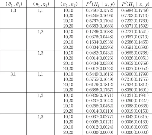
Example 1. To illustrate the Bayesian test procedures, we examine the cases when ( θ₁, θ₂) = (1,3),( 3, 1), ( η₁, η₂) = ( 1, 1), ( 1, 2), ( 1, 3) and ( n₁,n₂) = ( 5, 5)

, ( 5, 10), ( 10, 10),( 10, 20). The posterior probabilities of H₁ being true are computed assuming equal prior probabilities. The Table 1 shows that the results of the averages and the standard deviations in parentheses of posterior probabilities for each case based on 1,000 replications.

From the Table 1, when ( η1, η₂) = ( 1, 1), the fractional Bayes factor does not select H₁ for some small sample size cases. However the intrinsic Bayes factor gives fairly reasonable answers. Also for moderate sample sizes, the fractional and intrinsic Bayes factors give fairly reasonable answers.

Table 1: The averages and the standard deviations in parentheses of posterior probabilities

( θ₁, θ₂) ( η₁,η₂) ( n₁,n₂) P^F(H₁∣ x, y) P^I(H₁∣ x, y)

1,3 1,1 10,10

10,20 20,10 20,20

0.5491(0.1572) 0.6245(0.1696) 0.5767(0.1704) 0.6683(0.1683)

0.6984(0.1749) 0.7703(0.1713) 0.7232(0.1769) 0.8071(0.1592)

1,2 10,10

10,20 20,10 20,20

0.1786(0.1038) 0.0376(0.0448) 0.1634(0.0938) 0.0304(0.0296)

0.2721(0.1541) 0.0657(0.0713) 0.2686(0.1465) 0.0591(0.0590)

1,3 10,10

10,20 20,10 20,20

0.0482(0.0432) 0.0014(0.0026) 0.0404(0.0380) 0.0012(0.0023)

0.0865(0.0768) 0.0026(0.0051) 0.0852(0.0769) 0.0027(0.0052)

3,1 1,1 10,10

10,20 20,10 20,20

0.5449(0.1616) 0.5755(0.1649) 0.6179(0.1812) 0.6686(0.1757)

0.6900(0.1799) 0.7210(0.1755) 0.7624(0.1812) 0.8050(0.1691)

1,2 10,10

10,20 20,10 20,20

0.0826(0.1671) 0.0237(0.1042) 0.0258(0.0452) 0.0014(0.0110)

0.1021(0.1981) 0.0290(0.1227) 0.0368(0.0635) 0.0019(0.0153)

1,3 10,10

10,20 20,10 20,20

0.0037(0.0277) 0.0005(0.0121) 0.0012(0.0024) 0.0000(0.0000)

0.0042(0.0315) 0.0006(0.0139) 0.0016(0.0035) 0.0000(0.0000) Example 2. The data in Table 2 is taken from Bain and Engelhardt (1991).

Suppose a certain additive is proposed for increasing the length of time of tread wear of a tire. Suppose 40 of the present and 40 tires made under the new process are placed in service and the experiment is continued until the 20 smallest observations are obtained for each sample.

The value of fractional Bayes factor and arithmetic intrinsic Bayes factor of H2

versus H₁ is B^F₂₁= 0.1314 and B^I₂₁= 0.0563, respectively. We assume that the prior probabilities are equal. Then the posterior probability for H1 is 0.8839 and 0.9467, respectively. Thus there are strong evidence for H₁ in terms of the posterior probability.

Table 2: Length of time of tread wear Present

10.03 10.47 10.58 11.48 11.60 12.41 13.03 13.51 14.48 16.96 17.08 17.27 17.90 18.21 19.30 20.10 20.51 21.78 21.79 25.34

Additive

10.10 11.01 11.20 12.95 13.19 14.81 16.03 17.01 18.96 24.10 24.15 24.52 26.05 26.44 28.59 30.24 31.03 33.51 33.61 40.68

Example 3. The following data are a part of data which shows results of an experiment designed to compare the performances of high-speed turbine engine bearings made out of 5 different compounds (McCool 1979). The experiment tested 10 bearings of each type; the times to fatigue failure are given in units of millions of cycles. We did goodness-of-fit test of 5 types of data to 2-parameter exponential distribution and concluded that type II and type IV were accepted to this distribution. We used K-S statistic for the test.

Type II 3.19 4.26 4.47 4.53 4.67 4.69 5.78 6.79 9.37 12.75 Type IV 5.88 6.74 6.90 6.98 7.21 8.14 8.59 9.80 12.28 25.46

The value of fractional Bayes factor and arithmetic intrinsic Bayes factor of H2

versus H₁ is B^F₂₁= 12.771 and B^I₂₁= 10.0877, respectively. We assume that the prior probabilities are equal. Then the posterior probability for H1 is 0.0726 and 0.09019, respectively.

4. CONCLUSIONS

We developed a Bayesian test procedures for testing the equality of the difference of Guarantee time parameters in two parameter exponential distributions.

The refence prior is developed and posterior propriety is proved. Using this reference prior, the intrinsic Bayes factor of Berger and Pericchi (1996) and the fractional Bayes factor of O'Hagan (1996) are computed.

Through the simulation we can conclude that even for the small sample sizes, intrinsic Bayes factor performs better than the fractional Bayes factor. As the sample size grows large, the two Bayes factors perform reasonably. So, we recommend the use of intrinsic Bayes factors in this case.

APPENDIX 1. Derivation of the Reference prior and Propriety of the Posterior Distribution

Following Ghosal (1997) and Sareen (2003), we derive the reference prior of η, θ₁ and θ₂. The joint density is given by

f( x, y ∣η, θ₁,θ₂) = θ^{- n}₁ ¹θ^{- n}₂ ²exp { - n₁( x- η)

θ₁ - n₂( y- η) θ₂ }.

Now since l( η) = η,

c( η,θ₁, θ₂) = l '( η)f( l( η)∣η,θ₁, θ₂)

= θ^{- n}₁ ¹θ^{- n}₂ ²

= c₁(η)c₂(θ₁,θ₂),

where c1(η) = 1 and c₂( θ₁, θ₂) = θ^{- n}₁ ¹θ^{- n}₂ ². Moreover, letting θ = ( θ₁, θ₂),

J^{θ, θ} = E[ ∂

∂θ log f( x, y ∣η, θ)][ ∂

∂θ log f( x, y ∣η, θ)]'

=

[

]

Thus

detJ ^{θ, θ}(η,θ) = n₁n₂θ^{- 1}₁ θ^{- 1}₂

= λ₁(η)λ₂(θ),

where λ₁(η) = n₁n₂ and λ₂(θ) = θ^{- 1}₁ θ^{- 1}₂ . Therefore the reference prior η,θ₁ and θ₂. is given by

π( η, θ₁, θ₂)∝c₁(η) λ₂(θ) = θ^{- 1}₁ θ^{- 1}₂ .

Under this reference prior π(η,θ₁, θ₂) = θ₁^{- 1}θ₂^{- 1}, the joint posterior for η,θ₁ and θ2 given x, y is

π( η, θ₁,θ₂∣ x, y ) ∝ θ₁^{- n1- 1}θ₂^{- n2- 1}exp { - n₁( x- η)

θ₁ - n₂( y- η)

θ₂ }. (5) Integrating with respect to θ1 and θ2 in (5), then

π( η ∣ x, y) =C₁( x- η) ^{- n1}( y- η) ^{- n2}, η≤m _{x, y}. where m_{x, y}= min _{1≤i≤n1,1 ≤j≤n2}{x_i, y_j} and C₁ is a constant. Since

( x- η)≤( x- m_{x, y}) and ( y- η)≤( y- m _{x, y}), thus ⌠

⌡

mx, y

0 π(η∣ x, y )dη≤m _{x, y}( x- m_{x, y})^{- n1}( x- m _{x, y})^{- n2}. Thus the posterior distribution is proper if n₁≥1 and n₂≥1. This completes the proof. □

REFERENCES

1. Bain, L. J. and Engelhardt, M. (1991). Statistical Analysis of Reliability and Life-Testing Models, Marcel Dekker, New York.

2. Berger, J. O. and Bernardo, J. M. (1989). Estimating a Product of Means : Bayesian Analysis with Reference Priors. Journal of the American Statistical Association, 84, 200-207.

3. Berger, J. O. and Bernardo, J. M. (1992). On the Development of Reference Priors (with discussion). Bayesian Statistics IV, J. M.

Bernardo, et. al., Oxford University Press, Oxford, 35-60.

4. Berger, J. O. and Pericchi, L. R. (1996). The Intrinsic Bayes Factor for Model Selection and Prediction, Journal of the American Statistical Association, 91, 109-122.

5. Bhattacharya, S. K. and Srivastava, V. K. (1974). A Preliminary Test Procedure in Life Testing, Journal of the American Statistical

Association, 69, 726-729.

6. Chiou, P. and Han, C. P. (1989). Shrinkage Estimation of Threshold Parameter of the Exponential Distribution. IEEE Trans. Reliability, 38, 449-453.

7. Chiou, P. and Miao, W. (2004). Shrinkage Estimation for the Difference Between Exponential Guarantee Time Parameters. Computational Statistics and Data Analysis, in press.

8. Epstein, B. and Sobel, M. (1954). Some Theorems Relevant to Life Testing form an Exponential Populations. Ann. Math. Statist. 25,

373-381.

9. Epstein, B. and Tsao, C. K. (1953). Some Tests Based on Ordered Observations form Two Exponential Populations. Ann. Math. Statist., 24, 458-466.

10. Ghosal, S. (1997). Reference Prior in Multiparameter Nonregular Cases.

Test., 6, 159-186.

11. Ghosal, S. (1999). Probability Matching Prior for Non-regular Cases.

Biometrika., 86, 956-964.

12. McCool , J. I. (1979). Analysis of single classification experiments based on censored samples from the two-parameter Weibull distribution.

Journal of Statistical Planning and Inference, 3, 39-68.

13. O' Hagan, A. (1995). Fractional Bayes Factors for Model Comparison (with discussion), Journal of Royal Statistical Society, B, 57, 99-118.

14. O' Hagan, A. (1997). Properties of Intrinsic and Fractional Bayes Factors, Test, 6, 101-118.

15. Proschan, F. (1963). Theoretical Explanation of Observed Decreasing Failure Rate, Technometrics, 5, 375-383.

16. Sang Gil Kang and Hee Choon Lee (2004). Bayesian Test for the Intrass Correlation Coefficient in the One-Way Random Effect Model, Journal of Korean Data & Information Science Society, 15, 3, 645-654.

17. Spiegelhalter, D. J. and Smith, A. F. M. (1982). Bayes Factors for Linear and Log-Linear Models with Vague Prior Information, Journal of Royal Statistical Society, B, 44, 377-387.

[ received date : Sep. 2005, accepted date : Oct. 2005 ]