3-D Topology Optimization by a Nodal Density Method Based on a SIMP Algorithm

SIMP 기반 절점밀도법에 의한 3 차원 위상최적화

김 철^† · 팡 난^*

3-D Topology Optimization by a Nodal Density Method Based on a SIMP Algorithm

Cheol Kim and Nan Fang

Key Words : Topology optimization(위상최적화), SIMP(Solid isotropic microstructure with penalization), Nodal density(절점밀도), Finite element density(유한요소밀도)

Abstract

In a traditional topology optimization method, material properties are usually distributed by finite element density and visualized by a gray level image. The distribution method based on element density is adequate for a great mass of 2-D topology optimization problems. However, when it is used for 3-D topology optimization, it is always difficult to obtain a smooth model representation, and easily appears a virtual- connect phenomenon especially in a low-density domain. The 3-D structural topology optimization method has been developed using the node density instead of the element density that is based on SIMP (solid isotropic microstructure with penalization) algorithm. A computer code based on Matlab was written to validate the proposed method. When it was compared to the element density as design variable, this method could get a more uniform density distribution. To show the usefulness of this method, several typical examples of structure topology optimization are presented.

1. Introduction

The objective of the continuum structural topology optimization is to find out the optimum material distribution for a specified design domain, i.e., to find out an optimal load path between loading points and structural supports and provide an optimum distribution of materials after the minimization of structural compliance (i.e., maximization of stiffness). Since Bendsoe and Kikuchi ⁽¹⁾ suggested the basic theory of topology optimization based on the homogenization method in 1988, topology optimization design has been rapidly developed by in-depth study and extensive

research in terms of theories, methods and applications.

During the past two decades, plenty of topology optimization techniques have been proposed by many researchers. Zhou and Rozvany ⁽²⁾ and Zhou et al. ⁽³⁾ developed a so-called SIMP algorithm, which consider the element densities as the design variables and assume that material properties are constant within each element for discretizing the design domain. Eschenauer et al. ⁽⁴⁾ and Eschenauer and Schumacher ⁽⁵⁾ proposed an approach which is called the “bubble method”. In this method, some characteristic functions of the strains, stresses and displacements were used in order to find the placement or location of holes for a known shape at optimal positions, and consequently, a solution is obtained in a prescribed structural topology fashion.

Another approach so-called a level set method has been introduced into structural topology optimization by Sethian and Wiegmann ⁽⁶⁾. By this method, the structure

† Member, Professor

E-mail: [email protected]

Phone: (053)950-6586, Fax: (053)950-6550

* Graduate School, Dept. of Mechanical Eng, Kyungpook National University

대한기계학회 2008년도 추계학술대회 논문집

is represented by a level set model which is embedded in a scalar function. Xie and Steven ⁽⁷⁾ introduced an optimization method which is based on the evolutionary structural optimization approach. In the method, if the material in a design domain is not structurally active, it is considered as inefficiently used and can be removed by some element rejection criteria.

T

ue

v The SIMP (solid isotropic microstructure with

penalization) method has attracted some researchers interested in the topology optimization due to its simple concept and rapid implementation. It is also known as

“power-law approach”. The original SIMP method was introduced by Bendsoe ⁽⁸⁾, however, at that time it was expressed as a homogenization method under the name of “artificial density” or “the direct approach” in 1989. In the references ^{(2, 3)} a derivation of the SIMP method was also tried independently and the term SIMP was introduced first time in 1992. In the papers, a number of design conditions including stress constraints were applied. A similar approach was advocated by Mlejnek ⁽⁹⁾ and the SIMP method was coupled with the method of moving asymptotes. Sigmund ^{(10, 11)} and Sigmund and Petersson ⁽¹²⁾ discussed several drawbacks of the SIMP method including mesh-dependency, checkerboards patterns and local minima, and proposed a series of improvements by using mesh-independency filtering, higher order finite elements, a perimeter constraint and a gradient constraint.Bendsoe and Sigmund ^{(13, 14)} proved that the SIMP approach could be interpreted in physical terms as long as only the penalization power is a satisfied value. Pomezanski et al. ⁽¹⁵⁾ developed a so-called CO- SIMP algorithm based on the direct corner contact penalization to suppress the corner contacts problems.

In the SIMP method, material densities of all elements are considered to be constants and element relative densities are used as design variables to discretize a design domain. The final results of topology optimization are represented by a group of discontinuous step functions, which have the values between 1 (solid) and 0 (void). However, the problem is that these step functions have not afforded a smooth boundary layout unless an efficient finite element discretization technique is applied or a computational power improves through parallel computing ⁽¹⁶⁾, which, in turn, brings an expensive computational cost, especially for 3-D

topology optimization.

The objective of this study is to develop a simple and efficient method for 3-D topology optimization based on the SIMP method. Elements are connected by each node, and if the material densities are re-discretized from elements to nodes, a more uniform density distribution can be obtained. In this paper, discretized nodal densities were used to replace the element densities in order to obtain more uniform topology representation. The optimization procedure is established as following steps:

First, the 3-D design domain is discretized by eight-node hexahedron elements and each element density is calculated by the SIMP algorithm. Next, nodal densities are interpolated from the adjacent element densities by an element-to-node method ⁽¹⁷⁾. A computer code has been written to implement this pre-processing. The final topology result was visualized by Matlab for the element density case and by Tecplot for the nodal density case, respectively.

2. 3-D Topology Optimization Algorithm

2.1 SIMP algorithm

The design domain is discretized into a fixed grid of N finite elements and the design variables are constituted by the elements densities. The objective is to find an optimal material distribution subjected to some existent constraints. The minimization of a compliance function can be expressed as ⁽¹⁸⁾:

Minimize ₀ (1a)

1

( ) ^{T N} ( )_e ^p _e

e

cρ U KU ρ u k

=

= =

∑

Subject to ₀

1

( ) ^N _{e e}

e

V ρ V f ρ

=

= =

∑

KU= P ( ) 0

p

e e

k = ρ k

0<ρ_min ≤ ≤ρ 1 (1b)

where c( )ρ is the objective function to be minimized and and are a global displacement and a global stiffness matrix, respectively. is a global force vector, is an original element stiffness matrix, and are the element displacement vector and element stiffness matrix, respectively,

U K

P

k0 u_e k_e

ρ is the vector of design variables, and ρ is element densities, _e ρ_min is a lower limit of relative element densities but non-zero to avoid

matrix singularity, respectively. is the total number of elements and is the penalization power,

N

p V( )ρ

and are a material volume and a design domain volume,

(0) V

f is the prescribed volume fraction, and is an element volume.

ve

The optimizer is based on the standard optimality criteria method like Bendsoe ⁽¹⁹⁾. The Lagrangian function of Eq. (1a) can be expressed as:

0 0 1

( ) ( ) ( ( ) - ) ^T( - ) L ρ =c ρ λ+ V ρ fV +λ KU P

)

_{2 min 3 max} (2)

1 1

( ) (

N N

e e

e e

λ ρ ρ λ ρ ρ

= =

+

∑

∑

where λ and ₀ λ are the global Lagrangian multipliers ₁ , and λ and ₂ λ are Lagrangian multipliers for the ₃ lower and upper limit constraints. In order to find the stationary global point, Eq. (2) must satisfy the Kuhn- Tucker condition.

The sensitivity of the objective function can be obtained:

1

0 0

p T

e e

e e

c pρ u k u λ ^V

ρ ⁻ ρ

∂ = − = −

∂ ∂

∂

e

(3)

A heuristic updating scheme ⁽¹⁹⁾ for the design variables can be formulated as:

If ρ_eC_e^φ ≤max(ρ_min,ρ_e−m),

1 max( min, )

e m

ρ₊ = ρ ρ −

e

If max(ρ_max,ρ_e−m)<ρ_eC_e^φ <min(1,ρ_e+m) ρ_e+1=ρ_eC^φ If ρ_eC_e^φ ≥min(1,ρ_e+ m)

ρ_e+1=min(1,ρ_e+m) (4) where m is a positive move limit, φ is a numerical damping coefficient equals to 0.5 typically. m and φ can be varied from 0 to 1, and the purpose for introducing these two variables is to stabilize the iteration.

The stiffness matrix of the eight-node hexahedron element is given by

[ ]K =

∫ ∫ ∫

1 1 1

-1 -1 -1[ ] [ ][ ][ ]B^T D B J d d dξ η ζ

=

∫ ∫ ∫

where, is the strain-displacement matrix and is the shape function of the eight-node hexahedron element.

B N

2.2 Interpolation method

The nodal densities are interpolated from the adjacent element densities. It must be emphasized that in this paper the design variables are element densities different from the CAMD (continuous approximation of material distribution) method ⁽²⁰⁾ which used the nodal design variables. The resulting element densities are replaced by the relative nodal densities with an interpolation function.

The element-based SIMP method is used first to obtain the element densities distribution, and the node-based interpolation method is used later for getting the node densities distribution, so this case belongs to the element- to-node method.

The location relationship between the nodes and the elements is shown in Fig.1.

Fig.1 Illustration of location relationship between nodes and elements

All nodes in the design domain can be divided into four categories: (1) corner-node; (2) line-node; (3) surface-node; (4) body-node, which have the different number of adjacent elements. The node densities can be calculated as following ⁽¹⁷⁾:

1

1 nu

e e

n nu

e

v

v ρ ρ =

∑

∑

where ρ is the node density, _n ρ is the element density _e update from equation (1a), is the element volume, and is the number of adjacent elements, respectively. To simplify the Matlab code, here we assume that all elements have the same size, which is

ve

nu

very common in topology optimization by density distribution.

Corner node case: ρ_n =ρ₁e (7a) Line node case: 1 _{1 2}

2(

n e _e)

ρ = ρ +ρ (7b)

Surface node: 1 _{1 2 3 4}

( )

n 4 e e e e

ρ = ρ +ρ +ρ +ρ (7c)

Body node case: ¹( _{1 2} ... ₈

n 8 e e _e)

ρ = ρ +ρ + +ρ (7d)

2.3 Matlab implementation

A computer code using Matlab has been developed to implement all above process. All implementations are shown in following steps:

Step 1: Design domain initialization

Define the design domain as a 3-D matrix. The size of matrix is X×Y×Z. Consider the matrix elements to be the element densityρ . _e

Notice that volume constraint ₀

1

( ) ^N _{e e}

e

V ρ V f ρ v

=

= =

∑

and , so the element densities initialization values were defined with

0 1 N

e e

V

=

=

∑

f in the code.

Step 2: Calculate the FE stiffness matrix K.

Step 3: Calculate the displacement vector U. The supporting conditions and boundary conditions are defined in this part.

Step 4: Solve the objective function and sensitivity by a loop:

Objective function : ₀

1

( ) ^N ( )_e ^{p T}_e

e

c ρ ρ u

=

=

∑

Sensitivity equation : ¹ ₀

1

( )

N

p T

e e

e e

c p ρ u k

ρ ₌ ⁻

∂ =

∂

∑

Step 5: Sensitivity analysis by the mesh-independency filter by (4a), to ensure the existence of solution.

Step 6: Update the new element densities ρ_e+1 by the optimality criteria algorithm.

Step 7: Check the convergence of the result, If converges, go to next step. If not, return to step 4.

Convergence judgment method:

The change of the design variables (i.e. element densities): ρ_e+1−ρ_e< 0.05, convergence. Otherwise, un- convergence. The value 0.05 is prescribed and can be changed.

Step 8: Replace the element densities with the nodal densities by Eq. (6) and generate a Tecplot input-file.

Fig.2 shows an example of the input-file.

Fig. 2 Tecplot input-file fashion including: title, variables and data (partly).

3. Numerical Examples

The objective of topology optimization is to find the best material distribution, consequently establish a good foundation for the future shape optimization. In this section, two 3-D structural numerical examples are demonstrated in order to verify the efficiency of this method.

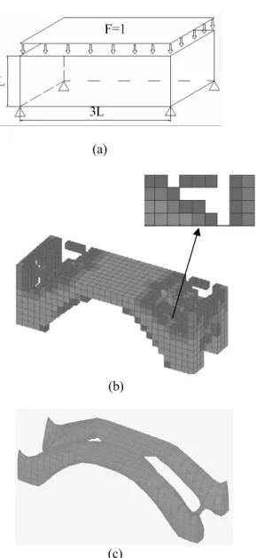
3.1 3-D brick structure

The design domain is shown in Fig. 3(a). A mesh of 20×10×10 elements is employed. The structure is fixed at the left surface of the domain and a vertical load is applied at the center of the right surface. Young’s modulus, E = 1 and Poisson’s ratio, ν = 0.3.

Figs. 3(b, c) show the topology optimization results by element and nodal density distributions, respectively. It is obvious that the new method provides a clear boundary than the previous method and can avoid the phenomenon of the virtual-connection in the low-density domain.

(a)

(b)

(c)

Fig. 3 (a) design domain for a 3-D brick, (b) topology result by element density distribution and the virtual- connect phenomenon, (c) topology result by node density distribution.

3.2 3-D bridge structure

In this section, the multiple-load case in 3-D topology optimization is shown. The design domain considered with corresponding applied distributed loads and boundary conditions is shown in Fig. 4(a). A mesh of 30 10 10 elements is employed and the material properties are the same as the previous model. The optimal results are shown in Figs. 3(b, c), respectively.

The topology material distribution of the case 2 is close to the realistic model obviously.

× ×

(a)

(b)

(c)

Fig. 4 (a) design domain for a 3-D bridge, (b) element density distribution and the low-density domain, (c) node density distribution

4. Conclusions

An efficient 3-D topology optimization method was developed based on the SIMP and the nodal density distribution of 3-D finite elements. The optimization procedure consists of major 2 steps: First, the 3-D design domain is discretized by eight-node hexahedron elements and each element density is calculated by the SIMP algorithm. Next, nodal densities are interpolated from the adjacent element densities by an element-to-node method A computer code has been developed to implement the algorithm. The final topology result was visualized by Tecplot based on the nodal density. When compared with

the traditional SIMP algorithm, the present method could obtain much smoother and clearer topology representation.

References

(1) Bendsøe, M. P., Kikuchi, N., 1988, “Generating Optimal Topologies in Structural Design using a Homogenization Method,” Comp. Meth. Appl. Mech.

Eng., Vol. 71, pp.197~224.

(2) Zhou, M., Rozvany, G. I. N., 1991, “The COC Algorithm, Part II: Topological, Geometry and Generalized Shape Optimization”, Comp. Meth. Appl.

Mech. Eng., Vol. 89, pp. 197~224

(3) Zhou, M., Rozvany, G.I.N., Birker, T. 1992:

“Generalized shape optimization without homogenization.” Struct. Optim, 4: 250~254.

(4) Eschenauer, H. A., Kobelev, H. A, Schumacher, A.

1994:“Bubble method for topology and shape optimization of structures.” Struct. Optim, 8: 142~151.

(5) Eschenauer, H. A., Schumacher, A. 1997: “Topology and shape optimization procedures using hole positioning criteria-theory and applications.” In:

Rozvany, G.I.N.(ed.) Topology optimization in structural mechanics, pp. 135~196. CISM Courses and Lectures, 374. Vienna: Springer

(6) Sethian, JA., Wiegmann A. 2000: “Structural boundary design via level set and immersed interface methods.” J. Comput. Phys, 163(2): 489~528.

(7) Y.M, Xie., and Steven, G.P. 1997: “Evolutionary structural optimization.” Springer-verlag, Berlin:

Springer.

(8) Bendsoe, M.P. 1989: “Optimal shape design as a material distribution problem”, Struct. Optim, 1:

193~202

(9) Mlejnek, H.P. 1993: “Some explorations in the genesis of structures.” In: Bendsoe, M.P., Mota Soares, G.A.(ed.) Topology design of structures (Proc. NATO ARW held in Sesimbra, 1992), pp. 287~300. Dordrecht:

Kluwer.

(10) Sigmund, O., 1994: “Design of material structures using topology optimization”, Ph.D. Thesis, Department of Solid Mechanics, Technical University of Denmark (11) Sigmund, O., 1997: “On the design of compliant mechanisms using topology optimization”, Mech. Struct.

Mach, 25: 495~526

(12) Sigmund, O., Petersson, J. 1998: “Numerical

instabilities in topology optimization: a survey on procedures dealing with checkerboards, mesh- dependencies and local minima.” Struct. Optim, 16:

68~75

(13) Bendsoe, M.P., Sigmund, O. 1999: “Material interpolation schemes in topology optimization.” Arch.

Appl. Mech, 69: 635-654.

(14) Bendsoe, M.P., Sigmund, O. 2003: “Topology optimization, theory, methods and applications”, Springer

(15) Pomezanski, V., Querin, O.M., Rozvany, G.I.N.

2005: “CO-SIMP:extended SIMP algorithm with direct corner contact control”. Struct. Multidisc. Optim, 30:

164~168.

(16) Borrvall, T., Petersson, J., 2001: “Large-scale topology optimization in 3D using parallel computing”, Computer Methods in Applied Mechanics and Engineering, 190: 6201~6229.

(17) Jin-Kyu, Byun., Joon-Ho, Lee., Il-Han, Park. 2004:

“Node-based distribution of material properties for topology optimization of electromagnetic Devices”.

IEEE Transactions On Magnetics, VOL. 40, NO. 2.

(18) Sigmund, O., 2001: “A 99 line topology optimization code written in Matlab”, Struct. Multidisc.

Optim, 21:120~127

(19) Bendsoe, M.P., 1995: “Optimization of structural topology, shape and material”. Berlin, Heidelberg, New York: Springer

(20) Matsui, K., Terada, K., 2004, “Continuous Approximation of Material Distribution for Topology Optimization,” International Journal for Numerical Methods in Engineering, Vol. 59, No. 14, pp. 1925~1944.