Prediction of the Fundamental Mode Lamb Wave Reflection from a Crack-Like Discontinuity Using Eigen-Mode Expansion

(1)

Prediction of the Fundamental Mode Lamb Wave Reflection from a Crack-Like Discontinuity Using Eigen-Mode Expansion

Jaeseok Park*^✝, Chang Heui Jang** and Jong Po Lee***

Abstract Based on the idea of eigen-mode expansion, a method to analyze the reflection of Lamb wave from a finite vertical discontinuity of plate is theoretically derived and verified by experiment. The theoretical prediction is in good agreement with the experimental result, and this strongly suggests that eigen-mode expansion method could be used for solution of inverse scattering problem for ultrasonic testing using Lamb wave.

Keywords: Lamb Wave, Eigen-Mode Expansion, Wave Refelection

Received: November 5, 2009. Revised: May 5, 2010; June 7, 2010, Accepted: June 10, 2010. *Corporate R&D Institute, Doosan Heavy Industries & Construction, 555 Guigok-dong, Changwon, Gyeong-nam, Korea, **Korea Advanced Institute of Science and Technology, 373-1 Guseong-dong, Yuseong-gu, Daejeon 305-701, Korea,

***ANSCO Corp., Jeonmin-dong, Yuseong-gu, Daejeon 305-811, ✝Corresponding Author: [email protected] Journal of the Korean Society

for Nondestructive Testing Vol. 30, No. 3 (2010. 6)

1. Introduction

Lamb wave was discovered by Horace Lamb in 1917 (Lamb, 1889; 1917). Currently, ultrasonic testing using Lamb wave is commonly being applied to evaluate the materials integrity of thin plate and or shell, since the Lamb wave propagates the plate with little ultrasonic attenuation. Time-consuming ultrasonic scanning process is not required accordingly (Alleyne et al., 1998). For the application of Lamb wave to nondestructive testing, physical understanding of interaction between Lamb wave and plate discontinuities and methods to quantitatively predict results of the interaction are needed (Alleyne and Cawley, 1992). For these purposes, various numerical methods such as boundary element method, finite element method, or hybrid solutions have been applied to predict scattering of Lamb wave (Cho and Rose, 1996).

Since the Lamb modes are the complete basis (Kirrmann, 1995; Bravdo, 1996), eigen-mode

expansion can be applied to analyze the interaction between Lamb wave and plate discontinuity. However, in previous studies (Torvik, 1967; Gazis and Mindlin, 1960;

Worlton, 1961; Lowe and Diligent, 2001), only reflection at the extremity of plate and vibration of circular disk were studied using eigen-mode expansion. These were due to difficulties to describe the boundary condition of finite vertical discontinuity. In this study, therefore, the necessities to investigate 1) reflection of the lowest anti-symmetric mode Lamb wave from a finite vertical discontinuity of plate by eigen-mode expansion and 2) its experimental verification are recognized.

2. Theoretical Development

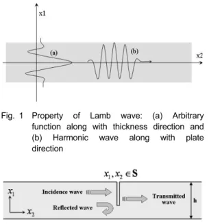
Lamb wave, which propagates the plate having stress free boundary, has typical characteristics of wave guide mode. In the direction of depth (_ in Fig. 1), particle

(2)

Fig. 1 Property of Lamb wave: (a) Arbitrary function along with thickness direction and (b) Harmonic wave along with plate direction

Fig. 2 Scattering geometry

velocity or stress has a form of arbitrary function, and in the direction of plate (_ in Fig. 1), there is a form of propagating wave;

 _ ^․^^^{  } ⁽¹⁾

where  and  are stress tensor and particle velocity vector by Lamb wave respectively,  is aritrary function,  is time, and  and  are wave number and angular frequency respectively which fulfill the Rayleigh-Lamb frequency equations;

 _

 _

 _^  ^^

^__

 (2)

 _

 _

 ^__

_^  ^^

 (3)

here, ^_^^^ ^ , ^_^^^ ^,  is the thickness of plate, _ and _ are wave numbers of longitudinal wave and transverse wave, respectively.

As shown in Fig. 2, once Lamb wave meets plate discontinuity, it is to be decomposed into

reflected wave and transmitted wave of which amplitudes are unknown. However, each scattered wave can be described by the linear series of Lamb modes, since the Lamb modes are complete basis;







∞

^{ }^{ }^^^ (4)







∞

^{ }^{ }^^^ (5) where   ± ± …, + and − correspond to positive direction and negative direction of wave respectively, ^ is weighting factor, ^^

is particle velocity, ^^ is stress for th Lamb mode of which wave number _ is th solution of eqns. (2) and (3). The time harmonic term

^ was dropped for simplicity.

At a discontinuity __∈, the sum of incidence wave and scattered wave should fulfill the boundary condition of which assumption is that a particle displacement and stress of each side of discontinuity are not continuous, and the surfaces of both side are stress free. This assumption is valid when the width of discontinuity is far smaller than the depth of the discontinuity but is larger than a particle displacement (Rokhlin, 1980). A tight crack-like discontinuity would be a good example for this boundary condition. So, boundary conditions of each part of discontinuity _  can be rewritten as

0 = ⁱⁿ+ ^rf where _ ∩_ , (6) 0 = ^trwhere _ ∩_ , (7) 0 = ⁱⁿ+ ^rf+ ^tr

where _≠ ∩_  ⁽⁸⁾ 0 = ⁱⁿ+ ^rf+ ^tr

where _≠ ∩_  ⁽⁹⁾ where superscript in, rf, and tr correspond to incidence wave, reflection wave, and transmission wave respectively.

(3)

) 0

( ) ( 21 21 +Σ⁻R ⁻ =

Σ^inc (16)

) 0

( ) ( 22 22 +Σ⁻R ⁻ =

Σ^inc (17)

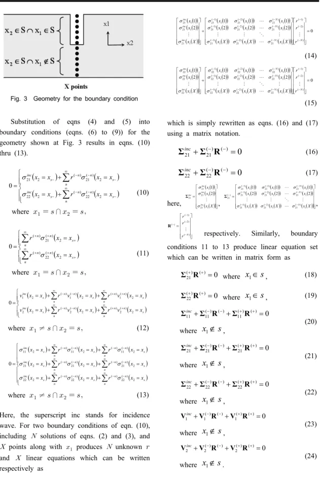
Fig. 3 Geometry for the boundary condition

Substitution of eqns (4) and (5) into boundary conditions (eqns. (6) to (9)) for the geometry shown at Fig. 3 results in eqns. (10) thru (13).

( ) ( )

⎪⎪

⎩

⎪⎪⎨

⎧

= +

=

= +

=

= ∑

∑

∞

−

∞

−

n

s n n s

inc

n

s n n s

inc

x x r

x x

x x r

x x

2 ) ( 22 ) ( 2

22

2 ) ( 21 ) ( 2

21

0

σ σ

where _ ∩_  

(10)

( )

⎪⎪

⎩

⎪⎪⎨

⎧

=

= ∑

∑

∞

+ +

+

∞

+ +

+

n

s n n n

s n n

x x r

2 ) ( 22 ) (

2 ) ( 21 ) (

0

σ σ

where _ ∩_  

(11)

( ) ( ) ( )

⎪⎪

⎩

⎪⎪⎨

⎧

= +

=

= +

=

= ∑ ∑

∑

∞ + +

∞ − −

∞ + +

∞ − −

n

s n n n

s n n s inc

n

s n n n

s n n s inc

x x v r x x v r x x v

2 ) ( 2 ) ( 2

) ( 2 ) ( 2

2

2 ) ( 1 ) ( 2

) ( 1 ) ( 2

1

0

where _≠ ∩_  (12)

( ) ( ) ( )

⎪⎪

⎪

⎩

⎪⎪

⎪

⎨

⎧

= +

=

= +

=

= +

=

∑

∞ − −

n

s n n n

s n n s inc

n s

n n

n s

n n s inc

n s

n n

n s

n n s inc

x x r x x r x x

2 ) ( 22 ) ( 2

) ( 22 ) ( 2

22

2 ) ( 21 ) ( 2

) ( 21 ) ( 2

21

2 ) ( 11 ) ( 2

) ( 11 ) ( 2

11

0

σ σ

σ

σ σ

σ

σ σ

σ

where _≠ ∩_  (13) Here, the superscript inc stands for incidence wave. For two boundary conditions of eqn. (10), including  solutions of eqns. (2) and (3), and

 points along with _ produces  unknown  and  linear equations which can be written respectively as

( ) ( )

( )

( ) ( ( )) ( ( )) ( )

( ) ( ( )) ( ( ))

2 0 2

2

1 1

1 2

1

) (

) 2 (

) 1 (

1 ) ( 21 1

) 2 ( 21 1 ) 1 ( 21

1 ) ( 21 1

) 2 ( 21 1 ) 1 ( 21

1 ) ( 21 1

) 2 ( 21 1 ) 1 ( 21

1 21

=

⎥⎥

⎥

⎦

⎤

⎢⎢

⎢

⎣

⎡

⎥⎥

⎥

⎦

⎤

⎢⎢

⎢

⎣

⎡ +

⎥⎥

⎥

⎦

⎤

⎢⎢

⎢

⎣

⎡

−

N N

inc inc inc

r r r

X x X

x X x

x x

x

x x

x

X x x x

M L

M O M M

L L

M

σ σ

σ

σ σ

σ

σ σ

σ

σ σ σ

(14)

( )

( ) ( ( )) ( ( ))

( )

( ) ( ( )) ( ( ))

( )

( ) ( ( )) ( ( ))

2 0 2

2

1 1

1 2

1

) (

) 2 (

) 1 (

1 ) ( 22 1

) 2 ( 22 1 ) 1 ( 22

1 ) ( 22 1

) 2 ( 22 1 ) 1 ( 22

1 ) ( 22 1

) 2 ( 22 1 ) 1 ( 22

1 22

=

⎥⎥

⎥

⎦

⎤

⎢⎢

⎢

⎣

⎡

⎥⎥

⎥

⎦

⎤

⎢⎢

⎢

⎣

⎡ +

⎥⎥

⎥

⎦

⎤

⎢⎢

⎢

⎣

⎡

−

N N

inc inc inc

r r r

X x X

x X x

x x

x

x x

x

X x x x

M L

M O M M

L L

M

σ σ

σ

σ σ

σ

σ σ

σ

σ σ σ

(15) which is simply rewritten as eqns. (16) and (17) using a matrix notation.

here,

( ) ( )

( ) ( )⎥⎥⎥⎥⎥

⎦

⎤

⎢⎢

⎢

⎣

⎡

= X x x x

inc inc inc

inc

1 21

21

2 1

σ σ σ Σ M

,

( )

( ) ( ( )) ( ( )) ( )

( ) ( ( )) ( ( ))⎥⎥⎥⎥⎥

⎦

⎤

⎢⎢

⎢

⎣

⎡

=

−

X x X

x X x

x x

x

x x

x

N N N

1 ) ( 21 1 ) 2 ( 21 1 ) 1 ( 21

1 ) ( 21 1 ) 2 ( 21 1 ) 1 ( 21 ) ( 21

2 2

2

1 1

1

σ σ

σ

σ σ

σ

σ σ

σ

L M O M M

L L Σ

,

⎥⎥

⎥

⎦

⎤

⎢⎢

⎢

⎣

⎡

=

−

) (

) 2 (

) 1 ( ) (

r N

r r R M

respectively. Similarly, boundary conditions 11 to 13 produce linear equation set which can be written in matrix form as

) 0

( ) ( 21⁺R⁺ =

Σ _wherex₁∈s_, (18)

) 0

( ) ( 22⁺R⁺ =

Σ _wherex₁∈s_, (19)

) 0

( ) ( 11 ) ( ) ( 11

11 +Σ⁻R⁻ +Σ⁺R⁺ =

Σ^inc

where x₁∉s_, ⁽²⁰⁾

) 0

( ) ( 21 ) ( ) ( 21

21 +Σ⁻R⁻ +Σ⁺R⁺ =

Σ^inc

where x₁∉s_, ⁽²¹⁾

) 0

( ) ( 22 ) ( ) ( 22

22 +Σ⁻R⁻ +Σ⁺R⁺ =

Σ^inc

where x₁∉s_, ⁽²²⁾

) 0

( ) ( 1 ) ( ) ( 1

1 +V⁻R⁻ +V⁺R⁺ =

V^inc

where x₁∉s_, ⁽²³⁾

) 0

( ) ( 2 ) ( ) ( 2

2 +V⁻R⁻ +V⁺R⁺ =

V^inc

where x₁∉s_. ⁽²⁴⁾

(4)

here, V1 and V2 of eqns. (23) to (24) are simply the matrix notation of corresponding boundary condition, eqns. (11) to (13). These nine matrix eqns. (16) to (24) can be assembled into global matrix form as

( )

( ) ( )

⎥⎦

⎢ ⎤

⎣

⎡

⎥⎥

⎦

⎤

⎢⎢

⎣

⎡

∉

∈

=

⎥⎥

⎦

⎤

⎢⎢

⎣

⎡

+

−

+

−

+

−

+

−

+

−

+

−

+ +

−

) (

1 ) ( 22 1

) ( 22

1 ) ( 21 1

) ( 21

1 ) ( 11 1

) ( 11

1 ) ( 2 1 ) ( 2

1 ) ( 1 1 ) ( 1

1 ) ( 22

1 ) ( 21 1

) ( 22

1 ) ( 21

22 21 11 2 1 22 21

0 0

R R

Σ Σ

V V

Σ Σ Σ

Σ

Σ Σ Σ V V Σ Σ

s x s x

s x

s x s x

s x

inc inc inc inc inc inc inc

(25)

which is simply rewritten as

T + MR = 0 (26)

using a matrix notation (e.g, ⁼^⎢_⎣^⎡ ⁺^⎥_⎦^⎤

− ) (

) (

R R R

and other in same way). R, the solution of linear matrix eqn. (26), can be calculated directly using the matrix identity;

(M M) M T

R= ^T ⁻¹ ^T (27)

where  and -1 are the transpose and inverse operator, respectively.

Since the energy carried by the Lamb mode of which wave number is th solution of Rayleigh-Lamb frequency eqns. (2) and (3) is defined as eqn. (28) (Morvan et al., 2003),

n n n

n r r P

E⁽⁾= ⁽⁾⋅ ⁽ ⁾^* _, (28) here, _ is acoustic Poynting vector of th Lamb mode (Auld, 1989). So the reflection index of  th Lamb mode defined as;

inc n n

E R E

) ) (

( = (29)

3. Numerical Implementation

At a given single frequency, finite number of real and imaginary solution, and infinite number of complex solution of Rayleigh-Lamb frequency

equation exist as shown in Fig. 4, and each solution corresponds to individual Lamb modes.

In real computation, it is not possible to include infinite number of Lamb mode to calculate the reflection, because the more numbers of Lamb modes are included into calculation, the larger size of matrix eqn. (25) and the more computation time are required. Thus, only reasonable numbers, which fulfill energy convergency is to be included;

∑

∑ ⁼

≅

n

inc n n

n

inc E R E

E ⁽⁾ ⁽ ⁾

or ∑ ⁽ ⁾≅1

n

Rn

.

(30)

In this study, 20 Lamb modes at 1.17 MHz·

mm and 200 points at a finite vertical discontinuity are included in the calculation.

Fig. 4 Complex solutions of Rayleigh-Lamb frequency equations; ‘*’ for anti-symmetric mode, ‘o’ for symmetric mode

Fig. 5 Experimental setup

(5)

Fig. 6 Example of A-scan for velocity measurement

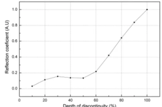
Fig. 7 Reflection amplitude of A0 mode Lamb wave from notches of 10~100% of through wall depth

Fig. 8 Theoretical prediction for reflection coefficients of A0 mode Lamb wave from finite vertical discontinuities of plate

4. Experiment

The experimental setup for Lamb wave reflection to verify the prediction by eigen-mode expansion is shown in Fig. 5. A single comb transducer of 1.55 mm pitch was used for both receiver and transmitter simultaneously. The center frequency and 6 dB bandwidth of ultrasonic transducer were 1.17 MHz and 30%

respectively. A reflection echo at the discontinuity was amplified before data acquisition system to increase the S/N ratio with 39 dB instrument gain. An EDM(electric discharge machinning) notched specimen was made of 1mm thick aluminum plate. The depth of notch ranged from 10% to 100%, and, the width and length of notch were 0.2 mm and 5 mm, respectively.

Fig. 6 shows the wave forms of reflection echoes from the plate extremity at two different positions of transducer. The path and time differences between two signals are 21.0 mm and 6.91 μsec which correspond to 3,039 m/s of wave velocity. This result confirms that the Lamb wave generated by the transducer was A0 mode.

The amplitudes of reflection echoes from EDM notches having variety of depth were measured. The experiments were performed 10 times to produce a deviation of measurement. At each individual measurement, all instruments were reset, and mechanical parts of the experimental setup were reassembled.

5. Results and Discussion

Fig. 7 is the experimental results which show reflection amplitudes vs. depths of notches. Fig.

8 shows the theoretical prediction. Both Fig. 7 and 8 showed similar trend that the reflection amplitudes did not simply increase as the depths of notches increased; (1) convex in the range of 0~50%, (2) depression near 50%, (3) linear in 50~100% with 0.186 and 0.194 of gradients respectively. Even though the experimental results showed a similar trend with theoretical one, the amplitudes showed a little differences in

detail; (1) theoretical result was concave but the experimental result was convex near 60% depth, (2) the depression of experimental result near 50% depth is not as sharp as one of theoretical prediction, and (3) 4.5% of gradient difference in 50~100%. In other word, the experimental result is smoother than the theoretical prediction. The Lamb wave impulse generated by comb transducer does not have single frequency 1.17 MHz, but have 30% of bandwidth. The

(6)

difference of two results may result from the bandwidth of incident A0 mode Lamb wave.

6. Conclusions

Based on the study of theoretical prediction by eigen-mode expansion and experiments to verify, followings were concluded;

(1) A method to analyze the reflection of Lamb wave from a finite vertical discontinuity was derived and experimental data were in good agreement with the theoretical prediction with a little differences in detail which may comes from the bandwidth of incidence A0 mode Lamb wave.

(2) The result strongly suggested that Eigen-mode expansion could be used for solution of inverse scattering problem for an ultrasonic testing using Lamb wave.

(3) For range of 50~100% through wall thickness, variation of reflection amplitude derived by Eigen-mode expansion could be utilized to estimate depth of discontinuity with 4.5% corrective factor.

(4) To estimate potential advantage in calculation time, comparing with a result by widely used CAE(computer aided engineering) tool can be suggested.

References

Alleyne, D. N., Cawley, P. (1992) Optimization of Lamb wave inspection techniques, NDT&E International, Vol. 25, pp. 11-22

Alleyne, D. N., Lowe, M. J. S. and Cawley, P.

(1998) The Reflection of Guided Waves From Circumferential Notches in Pipes, J. Applied Mechanics, Vol. 65, pp. 635-641

Auld, B. A. (1989) Acoustic Fields and Waves in Solids, 2nd Edition, Vol. 2, Krieger Publish- ing, USA Florida, p. 15

Bravdo, L. (1996) On the Stability of Lamb Modes, Acta Mechanica, Vol. 117, p. 71-80

Cho, Y. and Rose, J. L. (1996) A Boundary Element Solution for a Mode Conversion Study on the Edge Reflection of Lamb Waves, J.

Acoust. Soc. Am., Vol. 99, pp. 2097-2109

Gazis, D. C. and Mindlin, R. D. (1960) Extensional Vibrations and Waves in a Circular Disk and a Semi-Infinite Plate, J. Appl. Mech., Vol. 27, No. 4, pp. 541-547

Kirrmann, P. (1995) On the Completeness of Lamb Modes, Journal of Elasticity, Vol. 37, pp. 39-69

Lamb, H. (1889) On the Flexure of an Elastic Plate, Proc. London Math. Soc., Vol. 21, pp. 70-91

Lamb, H. (1917) On Waves in an Elastic Plate, Proc. Roy. Soc. London A, Vol. 93, pp. 114-128 Lowe, M. and Diligent, O. (2001) Reflection of the Fundamental Lamb Modes from the Ends of Plates, Review of Progress in Quantitive NDE, Vol. 20, pp. 89-96

Morvan, B. Wilkie-Chancellier N, Duflo H, Tinel A, Duclos J. (2003) Lamb Wave Reflection at the Free Edge of a Plate, J. Acoust. Soc. Am., Vol. 113, pp. 1417-1425

Rokhlin, S. (1980) Diffraction of Lamb Waves by Finite Crack in an Elastic Layer, J. Acoust.

Soc. Am., Vol. 67, pp. 1157-1165

Torvik, P. J. (1967) Reflection of a Rayleigh Wave from the Free End of a Waveguide, J.

Acoust. Soc. Am., Vol. 41, No. 2, pp. 346-353 Worlton, D. C. (1961) Experimental Confirma- tion of Lamb Waves at Megacycle Frequencies, J. Applied Physics, Vol. 32, pp. 967-971