Vol.34, No.2 pp. 131~136, 2010 (ISSN-1598-5725)
Inventory policy comparison on supply chain network by simulation technique
Nam-Kyu Park†․Woo-Young Choi*
†Department of Distribution Management, The Tong myung University, Busan, Republic. of Korea
* Department of Distribution Management, The Tong myung University, Busan, Republic. of Korea
Abstract : The aim of the paper is to solve the problem of customer reduction due to the difficulty of parts sourcing which impacts production delay and delivery delay in SC networks. Furthermore, this paper is to suggest the new inventory policy of MTS in order to solve the problem of current inventory policy. In order to compare two policies, a LCD maker is selected as a case study and the real data for 2007 years is used for simulation input. The maker uses MTO policy for parts sourcing which has the problem of lead time even if it has some advantage of inventory cost. Based on current process. The simulation program of AS-IS model and TO-BE model using ARENA 10 version is developed for evaluation. In a result, the order number of two policies shows that MTO is 52 and MTS is 53. However the quantity of order shows big difference such that MTO is 168,460 and MTS is 225,106. Particularly, the lead time of new inventory policy shows much shorter that that of MTO such that MTO 100 is days and MTS is 16 days. In spite of short lead time by MTS policy, new policy has to take burden of inventory cost per year. Total inventory cost per year by MTS policy is US $ 11,254 and each part inventory cost is that POL is US$ 1,807, LDI is US$ 2,166 and Panel is US$ 7,281. The implication of the research is that the company has to consider the cost and the service simultaneously in deciding the inventory policy. In the paper, even if the optimal point of deciding is put into tactical area, the ground of decision is suggested in order to improve the problem in SC networks.
Key words : SCM, Simulation, Arena, MTO, MTS
†Corresponding author: [email protected], 051)629-1861
* [email protected], 051)860-8844
1. Introduction
Supply chain management analyzes organically the whole process ranging from material supply to product delivery to the customers, checking and solving problems, and consequently trying to maximizing the profits of all the entities in a supply chain. To achieve effective and efficient supply chain management, the optimization of both production and inventory management of the organizations in the supply chain is greatly needed. Optimal production management and proper level of inventory lead not only to the cost reduction of the whole supply chain, but also to the profit increase of each individual company. Like this, an optimal production and inventory management policy is a critical factor to the success of supply chain management, but it is not an easy task. In order to achieve effective and efficient supply chain management, the level of inventory is required to remain to a minimum, reducing back-orders, and simultaneously maintaining a high service level. But inventory reduction and a high service level are contradictory to each other, and so, finding the best trade-off between these two goals is not an easy task. If exact forecasting is possible, we will be able to reduce inventory to a minimum, while fully satisfying customer‘s demand, but it is practically
impossible. This study has used two research methods theoretical research based on previous studies and simulation method. The previous studies are including literature review and theoretical research through the analysis of related data, while conducting expert interviews for related data collection.
Based on previous studies and related data, this study has designed both a production management model and an inventory management model, and then developed a simulation model. ARENA(Version 10) has been used as a simulation language. In order to observe inventory changes thoroughly, various order quantities and lead times have been used, and then we have analyzed their results.
2. Literature review
The research on the production planning under the MTO (Make-To-Order) production environment can be divided into two research at the strategic level and research at the operational level.
The researches at the strategic level are mainly focusing on the decision support system of corporate organizations in terms of a market environment. Carravilla & Sousaa (1995) have divided the production planning under the MTO environment of shoes industry into three stages and have
suggested a decision support system suite to the purpose of each stage. Corti et al. (2006) have checked the possibility of production according to the orders and delivery dates, and have suggested a model which enables the coordination of both production capacity and production range. Haskose et al.
(2004) have made researches on how much work volume affects the capacity of production system, mainly focusing on analyzing its effect in terms of material use and material procurement period. Giri and Yun (2005) have presented a model for determining opn aal production volume including the studies on production system failure and repairs which come from the uncertainty of production system. Bouchriha et al. (2005) have made researches on lot sizing in order to minimize the costs for the paper production process. Sphicas (2006) has intensified his studies on the existing EOQ (economic order quantity) model and EPQ (economic production quantity) model by adding the assumption on the permission range of backorder.
3. Case study of the selected company
The “A” company selected for this case study is a solid company located at Icheon of Gyeonggi Province. The reason why "A" company is selected as case study, is that "A" has been faced with difficult situation in terms of order lead time.
The company has been considering the new policy regarding to order process, production and inventory management. The company is producing about 60 items including the main products such as TFT-LCD(Thin Film Transistor-Liquid Crystal Display), LCD TV, Navigation and MP3 and 4. Its annual sales amount to about 100 billion Korean won. The company has another production base and logistics center in China, and 70% of the company’s total production comes from the first factory and the rest 30% from the second. The company is outsourcing its raw materials and parts to the outside companies. Therefore, it procures materials and parts from other partner companies, and manufactures its products through assembly lines, and produces its final products.
In this study we have selected one of its main products - a navigation module - for our case study, as it is practically impossible to use all the products for simulation test.
3.1 Case study of the selected company
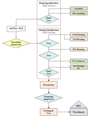
Let’s take a look at the production and logistics processes of “A” company. As shown in the <Figure 1>, it purchases materials such as a Glass, Pol, and LSI, and those items are to undergo the IQC(Incoming Quality Control) inspection and then move on to the panel production lines. After panel
production, module bonding, COG(Chip ON Glass), TCP (Tape Carrier Package), FPC(Flexible Printed Circuit) processes are to be followed. Again in-house inspections such as UV coating, air cleaning, and foil fixing are to be conducted and then go to the warehouse.
Fig. 1 “A” company’s production and logistics processes
3.2 Problems of logistics process
Through intensive and wide range of interviews with persons in charge of “A” company. This study has pointed out 9 kinds of problems such as “limited effectiveness of production planning”, “long lead time of main part” and “loss of customers due to delivery delay” These problems have been summarized in the below <Table 1>.
Table 1 “A” Company problems on business area
Production Planning
Limited effectiveness of production planning (production planning: once a month)
No simulation test because of production planning
Low yield of DSTN(Double Super Twisted Nematic) product
Production troubles (such as defective products) give rise to a material supply problem.
Materials Purchase
Long lead time of major parts (such as POL and IC)
Occurrence of a material supply problem gives rise to long waiting time, thus causing loss in job handling.
Lack of the proper linkage between parts order and final products delivery schedule
Product Delivery
Loss of customers due to delivery delay Occurrence of a production problem causes additional delivery costs due to emergency delivery.
4. Input data analysis of simulation modeling
In order to generate simulation input data, the following data for the selected product of “A” company have been collected for a full year from January 2007 to December 2007.
The interval of order arrival time, order quantity, order quantity of each part, and handling hours of production and each process. The collected data has been analyzed by Arena Input Analyzer.
Table 2 Manufacturing plant & delivery process simulation data
Section Expression
Order Recive -0.5 + LOGN(6.42, 6.01)’' Customer Order Amount NORM(3.74e+003, 1.66e+003) warehousing of Parts &
inspection Triangular(-0.5, 3, +0.5)
Produce Constant(5)
Finished product Triangular(±1, 2) Delivery to Customer Normal(±0.5, 2)
Table 3 Parts simulation data
Section Expression
Part Order
Panel: Order for the same amount of finished products LDI: Order for the same amount of finished products POL: Double order of finished products Panel Lead-Time Triangular(±1,2, 15) LDI Lead-Time Triangular(±1,2, 29) POL Lead-Time Triangular(±1,2, 31)
5. MTO simulation modeling
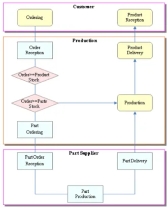
In order to define the MTO logistics process, this study has analyzed the production process of the “A” company as shown in the following <Figure2>. First of all, if the company receives an order, it will make production planning, while checking whether it has enough finished products or materials inventory for the order. If there are enough finished products. It will immediately deliver them to the customers, but if not, it has to place an order with outside companies for parts. In the case of parts, likewise, if it has enough parts inventory, it will soon start to manufacture, but if not, it has to place an order for parts. However, basically the MTO production method has no inventory of finished products or parts. Therefore, the above-mentioned process is not performed, but only for an exceptional case has its
process model been made the field workplace, 10% of additional parts order is being placed in consideration of the losses that can occur in the production or on the move. But this study is based on the assumption of having no loss. The parts such as panel, LDI, and POL will be supplied to the production line of the company, and according to its production planning, final products will be produced and inspected, and then delivered to the customers.
Fig. 2 MTO logistics process modeling
The performance of simulation has been conducted on a daily basis, and its results have been summarized on an annual basis. The simulation results of the MTO model are illustrated in the following <Table 4>. The differences between the current method and the MTO simulation model are as follows: the number of orders per year is 52, both are the same. In terms of annual order quantity, the current method amounts to about 194,000, and the MTO simulation model 211,000 showing a difference of 17,000. In terms of annual production volume, the current method amounts to 165,680, and the MTO simulation model 168,460, showing a difference of 2,780. In terms of the procurement period of purchase orders, the current method requires 96 days, and the MTO simulation model 100 day, showing the difference of 4 days. Finally, in terms of job performance rating within the delivery period, the former shows 88%, and the latter 89%. Based on these results, we can find out that the MTO simulation model is well reflecting reality.
Table 4 Present condition of production and MTO simulation result compare
Section
Annual Orders (Number)
Amount of Orders received
(EA)
Annual Production
(EA)
Lead-time (Day)
Deadline of Delivery
(%) Current
approach 52 194,464 165,680 96 88
MTO
Simulation 52 211,582 168,460 100 89
6. MTS simulation modeling
Ordering methods available in the MTS include quantity ordering, regular ordering, and Min-Max. In order to simplify the problem, this study has used quantity ordering, that is, EOQ and ROP (Re-Order Point).
6.1 MTS simulation input data
The collected data on the company’s main parts such as panel, LDI, and POL have been used as MTS simulation input data, which is shown in the following <Table 5>.
Table 5 MTS model basic input data
Section POL LDI Panel
Product price 0.5$ 2$ 8$
Stock
maintenance 20% 20% 20%
AVG Order
(1 times) 7,853(EA) 3,777(EA) 3,777(EA) Daily
Demand 1,1190(EA) 538(EA) 538(EA)
Deviation of
demand(Year) 503(EA) 242(EA) 242(EA)
Lead-Time
(AVG) 31(Day) 29(Day) 15(Day)
Ordering Cost 20$ 74$ 296$
By using the data on taking and placing orders during the past one year, this study has calculated EOQ and ROP, and its results are shown in the following <Table 6>.
Table 6 EOQ and ROP(each parts)
Section POL LDI Panel
Economic Order
Quantity(EOQ) 9,037 (EA) 8,525 (EA) 8,525 (EA) Reoder
Point(ROP) 41,209 (EA) 18,642 (EA) 10,255 (EA)
6.2 MTS inventory management model
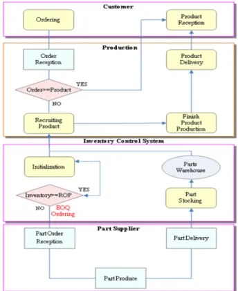
The MTS simulation model is much different than the MTO simulation model. As shown in the <Figure3>, the inventory control system has been operated independently,
not linked to other system. The inventory control system is based on the quantity ordering, always checking ROP, and placing an order by way of EOQ, if it goes below ROP.
Fig. 3 MTS logistics process modeling 6.3 MTS simulation results
The MTS simulation has been conducted on a daily basis.
In order to test the results and also to reduce the range of error, the simulations have been conducted for ten years. The results of simulations are shown in the following <Table 7>, which includes the number of orders per each time, quantity of orders fulfilled, production volume, average procurement period.
Table 7 MTS simulation result Section number
of orders Order
throughput Annual
production Lead-Time
AVG 53 53 225,106(EA) 16 (Day)
6.4 Inventory policy comparison between MTO & MTS This study has made a comparison of the results of both inventory policies. MTO inventory policy and MTS inventory policy. The results are as follows. In terms of the number of orders per year, MTO is 52, and MTS is 53. In terms of order quantity, both MTO and MTS show a similar result.
But in terms of annual production quantity, as shown in the
<Table 8>, MTO is 168,000 and MTS 225,106, showing a
difference of about 57,000. Meanwhile, in terms of procurement period, MTO is 100 days, and MTS is 16 days, making a great difference of 84 days. The reason is that, in the case of MTS inventory management model, it always has proper inventory available for every order, thus bringing productivity enhancement and reduction of procurement period.
Table 8 MTO & MTS simulation result comparison Section Annual
Order
Order Received
Annual Production
Lead-time (Day)
Deadline of Delivery
MTO 52 211,582 168,460 100 89%
MTS 53 225,106 225,106 16 100%
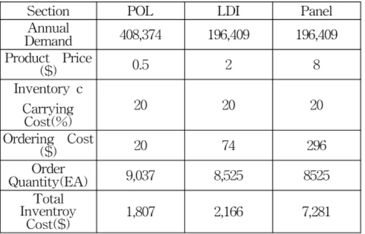
However, MTS increases inventory volume, which causes an inventory cost to increase, as illustrated in the <Table 9>.
Table 9 Annual inventory costs of each parts
Section POL LDI Panel
Annual
Demand 408,374 196,409 196,409
Product Price
($) 0.5 2 8
Inventory c Carrying
Cost(%)
20 20 20
Ordering Cost
($) 20 74 296
Order
Quantity(EA) 9,037 8,525 8525
Total Inventroy
Cost($) 1,807 2,166 7,281
Total inventory cost of each part can be calculated using following formula.
(1)
TC is the total annual inventory cost, I is item carrying cost(%/year), C is item cost, Q is order quantity(EOQ/EA), D and S is ordering cost($/EA).
7. Conclusions
This study has dealt with the SCM of domestic LCD module manufacturer, investigating how much the difficulty of parts procurement can affect production and delivery period, so that it may cause the loss of customers. So, this study has focused on solving this problem and simultaneously has tried to suggest the merits and demerits of a new alterative method.
This study has developed the MTO simulation system and MTS simulation system of the case company. By using both simulation models, we have compared and evaluated the results of both systems, presenting the problems to be solved and to be considered. According to the results of MTO inventory policy and MTS inventory policy, in terms of annual production quantity, MTO method is 168,460 and MTS method is 225,106 showing a difference of about 57,000 but in terms of procurement period, MTO is 100 days, and MTS is 16, making a great difference of 84 days. This great difference comes from the fact that MTS has proper inventory available for any order, consequently bringing productivity improvement and procurement period curtailment. In spite of this great achievement in terms of lead time, however, MTS has to bear considerable inventory costs in terms of inventory level.
Through this study the following lessons can be suggested. Business management is always facing continuous decision making process to choose a better alternative. In the case of an inventory problem, management has to make a decision on whether it will curtail inventory costs at the expense of customer service, or whether it will improve customer service at its expense.
Acknowledgements
This research was supported by Ministry of Knowledge and Economy, Republic of Korea, under the ITRC (Information Technology Research Center ) support program supervised by IITA(Institute for Information Technology Advancement) (IITA-2009-C1090-0902-0004)
References
[1] Altiok, T. and Melamed, B. (2007). "Simulation Modeling and Analysis with ARENA", Elsevier Science.
[2] Ballou, R.H. (1998). “Business Logistics Management, 4nd Edition”, Prentice Hall.
[3] Carravilla, M.A. and Sousaa, J.P. (1995), "Hierarchical production planning in a Make-To-Order company : a case study", European journal of operational research, Vol. 86, pp. 43~56.
[4] Corti, D., Pozzetti, A., and Zorzini, M. (2006), "A capacity-driven approach to establish reliable due dates in a MTO environment ", International Journal of Production Economics, Vol. 104, pp. 536∼554.
[5] Giri, B.C. and Yun, W.Y. (2005), “ Optimal design of unreliable production–inventory systems with variable
production rate ”, European Journal of Operational Research, Vol 162, pp. 372∼386.
[6] Haskose, A., Kingsman, B.G., and Worthington, D.
(2004), "Performance analysis of make-to-order manufacturing systems under different workload control regimes" International Journal of Production Economics, Vol 90, pp. 169∼186.
[7] Simchi-Levi, D., Kaminsky, P., and Simchi-Levi, E.
(2003). “Designing & Managing the Supply Chain, 2nd Edition", McGraw-Hill.
[8] Sphicas, G.P. (2006), "EOQ and EPQ with linear and fixed backorder costs: Two cases identified and models analyzed without calculus", International Journal of Production Economics, Vol 100, pp. 59∼64.
Received 2 September 2009 Revised 9 March 2010 Accepted 17 March 2010