A Sensitivity Analysis of the Optimal Inventory Control for a Vertically Integrated Supply Chain

Vol. 30, No. 3, pp. 197-204, September 2004.

A Sensitivity Analysis of the Optimal Inventory Control for a Vertically Integrated Supply Chain

Engab Kim

College of Business Administration, Ewha Womans University, Seoul, 120-750

수직적으로 통합된 공급사슬을 위한 최적 재고 정책의 민감도 분석

김 은 갑

이화여자대학교 경영대학

This paper deals with a supply chain with a company and its contractor that produces products by the OEM contract with the company. The supply chain of interest has two distinct features. First, the company is the supplier of raw material required in the production at the contractor. Second, the company and its contractor make a delivery shipment arrangement that the replenishment lead time is determined depending on demand process. We show that the optimal inventory policy is monotonically changed as either the replenishment setup cost or inventory holding cost becomes increased or decreased. We also present asymptotic properties of the optimal inventory policy when either the number of outstanding customer orders or the inventory level becomes very large.

Keywords: supply chain management, OEM, inventory management, sensitivity analysis

The work of the author was supported by Ewha Womans University under Grant No.110-20030008.

†Corresponding author : Professor Eungab Kim, College of Business Administration, Ewha Womans University, Seoul, 120-750, Fax +82-3277-2776, E-mail [email protected]

Received February 2004; revision received May 2004; accepted May 2004.

1. Introduction

This paper considers a supply chain model with a company and its contractor that produces products by the OEM(original equipment manufacturer) contract with the company. In today’s business world, it is one of the major issues how to realize an integrated corporation that allows a company to work closely with internal business partners(National Academy Press, 1999). Companies with effective partnerships have advantages over supply chains owned by a single company because they are capable of building or dissolving those partnerships quickly according to the market condition(Fry et al., 2001; Simchi-Levi, 2000).

This paper deals with the inventory management

when the company is the supplier of raw material required in the production at the contractor. A raw material replenishment process between these two companies is described as follows. The company receives an order from a customer and transmits it to the contractor. If there are no orders in production queue, the contractor allocates raw material in inventory and produces the product for that customer.

If there are orders in process, the production of this order is delayed until preceding orders are all served.

Upon the production completion, the contractor initiates a delivery process to that customer and this information is feedback to the company. Based on it, the company activates a billing process and the order is closed.

In this paper, we assume that these two companies

make a contract that lead time for inventory replenishment is determined depending on demand process. Most of inventory models in the literature (Axsäter, 1993; He et al., 2002; Silver and Peterson, 1985) have dealt with a replenishment lead time that is quoted by either side of supply and demand at the time when an order is placed (or received). In general, it is assumed to be given into the modeling. In the model of interest, however, neither the company nor the contractor quotes lead time but they have a prescribed shipment rule working as follows. Upon receiving a replenishment order from the contractor, the company does not begin a shipment of raw material to the contractor until a certain number of customer orders are recorded since the order place- ment. Hence, the length of lead time becomes increas- ed or decreased depending on demand process.

The model studied in this paper was introduced by Kim(2004). In Kim(2004), he characterized an optimal policy controlling the raw material flow between two companies under the demand dependent shipment strategy and numerically showed that this strategy could be beneficial to the entire supply chain.

This result indicates that there could be considerable gains from being able to observe more demands before assigning inventory to the contractor. For example, if there is a momentary lull in the market after the inventory decision, the proposed shipment strategy allows the replenishment lead time to become increased, and thus the contractor can avoid inventory burden. The detailed discussion about the demand dependent shipment strategy can be found in Kim (2004).

The goal of this paper is to present a sensitivity analysis for the optimal inventory control that was identified in Kim (2004). We analyze how the optimal inventory cost and optimal inventory policy change as some of system parameters increases or decreases.

Especially, we establish a monotonicity of the optimal inventory policy with respect to system costs. The problem presented here falls in the category of optimal control of queueing systems. There are few reports about the marginal analysis of the optimal control policy. Carr and Duenyas(2000) and Van Oyen(1997) performed a marginal analysis similar to ours with different problems. We also present the asymptotic properties of the optimal inventory policy that can be useful in developing heuristic policies that are applicable to the real world problems. Koole(1997) and Ha(1997) identified asymptotic optimal properties of the switching control policy for server allocation in the multi-class queueing system and applied their results to developing heuristic policies. Although the model considered in this paper is simple, we hope that the results obtained here can give insights into more

complex supply chain models.

The rest of the paper is organized as follows. In the next section, we define a Markov decision problem (MDP) formulation of our model. The sensitivity analysis is presented in Section 3. Section 4 identifies asymptotic properties of the optimal inventory policy.

Finally, in Section 5, results obtained in this paper are summarized and future research is discussed.

2. Model Definition

For the sake of the discussion, we present a curtail- ment of the problem formulation section in Kim (2004). In this paper, however, we assume zero transportation time from the company to the contrac- tor. It is important to note that our sensitivity analysis can be extended to the model with exponential transportation times that is considered in Kim (2004).

In fact, the sensitivity analysis for the model with exponential transportation times has the same functio- nal properties as presented in this paper but it requires more or less complicated and lengthy mathematical steps for the proof.

Customer orders with equal order size arrive at the company according to a Poisson process with rate

λ > 0 . Without loss of generality, one unit of raw material is used when the contractor processes each customer order. Production times are exponential random variables with mean _μ

and successive productions are independent of all else.

This paper assumes a replenishment shipment arrangement in which the company initiates a delivery of raw material after N additional customer orders are recorded since a replenishment order from the contractor. The transportation time from the company to the contractor is assumed to be negligible. Under this shipment rule, the replenishment lead time D is given by D = ∑

i = 1

D

where _D

’s are i.i.d. exponentially distributed with rate _λ . _D

’s can be considered as the replenishment process phases that are performed in sequence.

The cost structure of the model is as follows: A

linear cost _c is assessed for each unit of time for each

outstanding customer order while a linear cost _h is

incurred for each unit of time for each unit of raw

material in inventory. The cost c can be viewed as

providing an incentive to minimize the weighted flow

times of customer orders. There is a lump-sum

replenishment setup cost _K at each instant a

replenishment order is placed. The order quantity, _Q ,

is given and constant.

The original problem is a continuous Markov decision problem (MDP) and, by following the uniformization process in (1987), it can be converted into an equivalent discrete time MDP with a transition rate _{γ ≜ λ + μ} and the discount factor ^γ

β + γ where _β is a discount factor for the continuous MDP. Without any loss of generality, we scale the time unit so that

β + γ = 1 .

A state is described by the vector ( x , y , n) where x and _y denote the number of customer orders in queue and the raw material inventory level, respecti- vely. And _n is an indicator: if _{n = 0} , no replenish- ment orders are in process; if _{1 ≤ n ≤ N} , an order is in process and _{N - n} customer orders are observed since the order placement.

The set of decision epochs consists of customer order arrival and production completion epochs. An inventory policy specifies, at each decision epoch, whether or not the contractor places a replenishment order. We assume that the replenishment order is never interrupted until it arrives at the contractor.

Therefore, for state _{( x, y, 0)} , there are two admissi- ble actions : Do not replenish and Replenish.

The goal of this paper is to find an inventory control policy that minimizes the total expected discounted costs over an infinite horizon. Define J( x, y, n) to be the optimal expected discounted cost over an infinite horizon given the initial state _{( x, y, n)} . Then,

J( x, y, n) can be shown to satisfy the following optimality equation:

J( x, y, n) = _{min T}

_J(x,y,n),T

_{J( x,y, n)} (1) _{if n = 0}

_T

_J(x,y,n) if 0 < n ≤N

where

T

J(x,y,n) =

cx + hy + λJ( x + 1, y, 0) + μJ( D( x, y),0)

_{if n = 0} cx + hy + λJ( x + 1,y,n - 1)+ μJ( D( x, y),n)

if 1 < n≤N

cx + hy + λJ( x + 1, y + Q, 0)+ μJ( D( x, y),1)

_{if n = 1}

T

J( x,y, 0) = K + T

J(x,y,N),

and D( x, y) = ( x - 1, y - 1) if _{x >} 0 and y > 0; other- wise, _{( x,y)} . We note that _T

and _T

are value iteration operators corresponding to the actions of Do not replenish and Replenish action, respectively.

3. Monotonicity of the Optimal Per- formance with Respect to System Parameters

To help the understanding of the sensitivity analysis, we introduce the optimal inventory policy identified in Kim (2004). For the detail of the analysis, please refer to Kim (2004).

Theorem 1 (i) Let

r( x) : = max {y ∈ {0, 1,…,∞ } : T

J( x, y, 0)

_{< T}

_{J(x,y,0) }} (2) Given _x and _y , it is optimal for the company to initiate a replenishment process if the current inventory level at the contractor, _y , drops to or below

r( x) .

(ii) The threshold function _{r( x)} increases as the size of outstanding customer orders, _x , also increases;

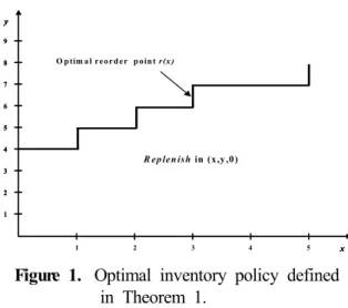
r( x) ≤ r ( x + 1), x ≥ 0. (3) The optimal inventory policy characterized by Theorem 1 can be viewed as a dynamic version of

( Q, r) policy. The first part of Theorem 1 states that the optimal inventory reorder point for the contractor is given as a function of both the number of outstanding customer orders _x and the inventory level

y and has a threshold structure. The second part of Theorem 1 says that the optimal inventory policy has a monotonicity. That is, it is optimal to place a replenishment order only when the number of outstanding customer orders exceeds a threshold value, given the inventory level, and it is increasing as the inventory level increases. <Figure 1> graphically represents such an optimal inventory policy.

Figure 1. Optimal inventory policy defined in Theorem 1.

x y

xx yy

1 2 3 4 5

2 4 5 6 7 8 9

1 3 2 4 5 6 7 8 9

1 3

R ep len ish in (x,y ,0) O p tim a l reord er p oin t r(x)

{

We now proceed to analyze how the optimal cost and optimal inventory policy change as a function of system parameters. We first set the monotonicity of the optimal discounted cost J as a function of system parameters such as the production rate μ, outstanding customer order cost c, inventory holding cost h, and replenishment setup cost K, given the order quantity.

The following is an intuitive result.

Theorem 2 The optimal cost function J( x, y, n) is decreasing in _μ and increasing in _c , _h , and _K .

Proof of Theorem: Suppose we reduce _c , _h , and

K . The changes in _c , _h , and _K guarantee lower costs if the policy which is the optimal before the change is also applied after the change is made. We now give the proof for _μ . Consider two systems, labeled system _A and system _B , that are identical except for the service rates _μ

and _μ

where

μ

< μ

. Let _π

be the optimal policy applied to system _A . For each service in system _B , we employ

π

allowing for idling for the period of _μ

_{- μ}

appropriately along each sample path to make the evolution of system _B identical to that of system _A under _π

. It is clear that the policy _π

results in the equal performance to _π

. Because _π

may not necessarily be optimal, the optimal policy in system

B will perform at least as well _π

.

We next proceed to identify the monotonicity of the optimal inventory policy defined in Theorem 1 with respect to the replenishment setup cost _K and inventory holding cost h given the order quantity. In other words, we show how the optimal reorder point r(x) is monotonically changed as each of these costs is increased or decreased.

Consider two instances of the problem described by (1). To differentiate each other, we use symbol _A and

B in the first and second case, respectively, for the system parameters, optimal cost function J, and optimal inventory policy r(x). We first present the sensitivity analysis for the replenishment setup cost

K . Suppose that _K

_{< K}

.

Consider the following functional properties esta- blished by the optimal inventory costs _J

and _J

:

J

(x,y,0) - J

(x,y,N) ≤ J

(x,y,0) - J

(x,y,N)

_{+ K}

_{- K}

_, (4)

J

(x,y,n+ 1) - J

(x,y,n) ≤ J

(x,y,n + 1)

_{- J}

(x,y,n), n ≥ 1, (5)

J

(x,y,1) - J

(x,y + Q,0) ≤ J

(x,y,1)

- J

(x,y+ Q,0) , (6)

J

(x+ 1,y+ 1, n) - J

(x,y,n) ≤ J

(x+ 1,y+ 1, n)

_{- J}

(x,y,n), n ≥ 0. (7)

We first provide the following lemma:

Lemma 1 If (4)-(7) hold,

T

J

(x,y,0) - T

J

(x,y,0) ≤ T

J

(x,y,0)

- T

J

(x,y,0). (8)

Proof:

T

J

(x,y,0) - T

J

(x,y,0) - ( T

J

(x,y,0)

_{- T}

_J

(x,y,0)) =- K

+ K

_{+ λ[ J}

(x+ 1,y,0) - J

(x+ 1,y,N - 1)

_{- ( J}

(x+ 1,y,0) - J

(x+ 1,y,N - 1))]

_{+ μ[ J}

(D(x,y),0 ) - J

(D(x,y),N )

_{- ( J}

(D(x,y),0 ) - J

(D(x,y),N ))]

_{≤ - K}

_{+ K}

_{++ λ[ J}

_{(x+ 1,y,0) - J}

(x+ 1,y,N) - ( J

(x+ 1,y,0) _{- J}

(x+ 1,y,N) )]

_{+ μ[ J}

(D(x,y),0 ) - J

(D(x,y),N )

_{- ( J}

(D(x,y),0 ) - J

(D(x,y),N ))]

(by (5))

_{≤ - K}

_{+ K}

+ ( λ + μ)( K

- K

)

( by λ + μ ≤ 1)

(by (4)) ≤ 0 ( by λ + μ ≤ 1).

Suppose that it is optimal not to replenish in state

( x, y, 0) under system A, that is, _T

_J

(x,y,0) <

T

J

(x,y,0) . Then, by (8) in Lemma 1, _T

_J

_(x,y,0)

< T

J

(x,y,0) , which implies that the optimal policy should not replenish in state _{( x, y, 0)} under system B. This result can be explained by the fact that System B has a larger replenishment setup cost than System A.

Next, we show that (4)-(7) are preserved under the value iteration operator _T .

Lemma 2

(i) _TJ

(x,y,0) - TJ

(x,y,N) ≤ TJ

(x,y,0)

_{- TJ}

(x,y,N) + K

- K

(ii) _TJ

(x,y,n+ 1) - TJ

(x,y,n) ≤ TJ

(x,y,n+ 1)

_{- TJ}

(x,y,n), n ≥ 1

Figure 2. Optimal inventory policy as a function of the replenishment setup cost K.

5 10 15 20

5 10 15

K=100 K=150 K=200

x y

(iii) _TJ

(x,y,1) - TJ

(x,y+ Q,0)

_{≤ TJ}

(x,y,1) - TJ

(x,y+ Q,0) (iv) _TJ

(x+ 1,y+ 1, n) - TJ

(x,y,n)

_{≤ TJ}

(x+ 1,y+ 1, n) - TJ

(x,y,n) Proof : See the Appendix

By Lemma 1 & 2, we can present the monotonicity of the optimal inventory policy with respect to the replenishment setup cost K as follows :

Theorem 3 Suppose that _λ

_{= λ}

, _μ

_{= μ}

, _c

₌ c

, _h

_{= h}

, and _K

_{< K}

. Then, _r

_{(x) ≥ r}

_(x) for all _{x ≥ 0.}

Proof : We prove _r

_{(x) ≥ r}

_(x) using contradic- tion. Suppose _r

_{(x) < r}

_(x) . Then, we have _T

_J

( r

(x),y,0) ≥ T

J

(r

(x),y,0) and _T

_J

_(r

( x), y, 0) < T

J

(r

(x),y,0) . It follows that _T

_J

( r

(x),y,0) - T

J

(r

(x),y,0) < T

J

(r

(x), y, 0) < T

J

(r

(x),y,0) - T

J

(r

(x),y,0) , which is a contradiction by (8) of Lemma 1.

If systems A and B are identical with respect to the system parameters except that System B has a larger replenishment setup cost than System A, Theorem 3

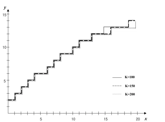
states that the optimal reorder point of System A is equal to or higher than that of System B. Theorem 3 can be extended to the following more generalized result: as the replenishment setup cost K increases, the optimal policy more restricts replenishing inventories in any given state _{( x, y, 0)} .

Such behavior of the optimal policy has some interesting features. The result of Theorem 3, _r

_{( x)}

≥ r

(x) , means that if both systems have the same inventory level, System B delays a replenishment decision until more customer orders arrive while System A immediately places a replenishment order.

In other words, the increase in the replenishment setup cost may push the optimal policy to incur more production delay costs in order to avoid frequent replenishment orders. <Figure 2> displays how the optimal inventory policy changes as a function of _K for the example with _{c = 3} , _{h = 1} , _{λ = 0.6} , _{μ = 1} ,

Q = 20 .

The monotonicity of the optimal inventory policy with respect to the inventory holding cost _h is also identified in the following theorem. Since the proof of Theorem 4 is similar to that of Theorem 3, we omit the proof of it.

Theorem 4 Suppose that _λ

_{= λ}

, _μ

_{= μ}

,

d

= d

, _K

_{= K}

, _c

_{= c}

, and h

< h

, Then,

r

(x) ≥ r

(x) for all _{x ≥ 0} .

Suppose that systems A and B are identical with respect to the system parameters except that System B has a larger inventory holding cost than System A.

Then, Theorem 4 states that the optimal reorder point of System A is equal to or higher than that of System B. Theorem 4 can be extended to the following more generalized result: as the inventory holding cost h increases, the optimal policy more restricts repleni- shing inventories in any given state _{( x, y, 0)} .

The result of Theorem 4, _r

_{(x) ≥ r}

_(x) , means that if both systems have the equal number of outstanding orders, System B delays a replenishment decision until more inventory is dedicated to the production while System A immediately places a replenishment order. Such an optimal behavior of System B may incur more production delay of customer orders because the possibility of stock out can increase. Nonetheless, the increase in the inventory holding cost justifies the optimal policy to delay the replenishment order in order to avoid large inventories.

4. Asymptotic Properties of the Optimal Inventory Policy

The value iteration method is mostly used to find an optimal control policy in the area of the control of queueing network. Since the state space of the problem described by (1) is infinite, it is necessary to truncate the state space. Therefore, we need to approximate the optimal cost function _J along and beyond the boundaries the truncated state space. This section presents the asymptotic properties of _J under an optimal inventory policy that can be used as an approach to the approximation. We first introduce the following first difference functions:

∆

J(x

x

n) = J( x

+ 1,x

n) - J( x

x

n),

∆

J(x

x

n) = J( x

x

n + 1) - J( x

x

n).

Operators ∆

and ∆

implies the marginal cost of holding one more customer order in queue and one more unit of raw material in inventory, respectively.

The following theorem defines an asymptotic property of the optimal cost function _J when the number of outstanding customer orders are very large.

That is, it says that the optimal cost function _J is asymptotically linear.

Theorem 5

lim

∆J(x,y,n) = c

1 - γ , 0 ≤n ≤N. (9) Proof: See the Appendix

Equation (9) implies that if _x goes to the infinity, the optimal actions applied to states _{( x, y, 0)} and

( x + 1, y, 0) are the same, which means that the optimal inventory policy does not depend on _x .

In the following, we provide an asymptotic property of the optimal cost function _J with respect to the inventory level _y. Theorem 6 implies that the optimal inventory policy does not depend on _y if it goes to the infinity. It can be proven using an argument similar to one in Theorem 5 and thus we omit the proof of it.

Theorem 6

lim

∆

J( x, y, n) = h

1 - γ , 0 ≤ n ≤ N. (10) Using the result of Theorem 5 and Theorem 6, the following approximations of the optimal cost function J along the boundary of the truncated state space can be obtained:

J( M,y,n) = J( M - 1, y, n) + c 1 - γ , J( x,W,n) = J( x,W - 1,n) + h

1 - γ

where M and W are some positive integer.

The intuition of Theorem 5 and 6 is as follows.

Suppose that there are very large inventories at the contractor. Having one more unit of raw material incurs an addition cost of _h over the time until excessive inventory has been depleted. In the limit, the net present value of this additional cost becomes

h ⌠ ⌡

∞

0

e

dt = h /( 1 - γ). We can provide a similar interpretation for the outstanding customer order case.

5. Conclusion and Future Research

This paper considered a supply chain model with the

demand dependent shipment rule which was presented

in Kim(2004). Under the assumption of zero trans-

portation time, we implemented the sensitivity analysis

of the optimal inventory policy, characterized in Kim

(2004), with respect to the system parameters. In

particular, we were able to show that the optimal

inventory policy is monotonically changed as either the replenishment setup cost or inventory holding cost becomes increased or decreased. The sensitivity analysis obtained in this paper can be extended to the case with exponential transportation times.

Many open problems remain to be explored. First, our formulation can extend to general distributions other than exponential distribution. Incorporating Erlang demand inter-arrival, production, or transpor- tation times into the model will be an important research topic because it allows us to investigate the impact of their variance on the optimal inventory policy and the sensitivity analysis. Second, it is unresolved to show the monotonicity of customer order arrival process on the optimal cost and customer order waiting cost on the optimal inventory policy.

Finally, to develop heuristic policies using the marginal and asymptotic properties identified in this paper will be another future research topic.

Appendix

Proof of Lemma 2 : Denote by _{( u}

_/p

₎ the optimal action for the first instance where _μ

and _p

represent Do not replenish and replenish actions, respectively. Similarly, ( u

/p

) correspond to the second instance.

(i) _TJ

(x,y,0) - TJ

(x,y,N) ≤ TJ

(x,y,0) - TJ

(x,y,N) + K

- K

:We focus on admissible actions in _(x,y,0)

and _(x,y,0)

. Case _{( p}

_{, u}

₎ is excluded by Lemma 1. For ( p

, p

) , from the definition _T

_J,T

_J

(x,y,0)-T J

(x,y,N) - ( T

J

(x,y,0)

- TJ

(x,y,N)) = K

- K

.

For ( u

, u

) , T

J

(x,y,0) - TJ

(x,y,N) -

( T

J

(x,y,0) - TJ

(x,y,N)) ≤ T

J

(x,y,0)

- TJ

(x,y,N) - ( T

J

(x,y,0) - TJ

(x,y,N))

(by Lemma 1) = K

K

.

For _{( u}

_{, p}

₎ ,

T

J

(x,y,0) - TJ

(x,y,N) - ( T

J

(x,y,0) - TJ

(x,y,N)) ≤ T

J

(x,y,0) - TJ

(x,y,N) - ( T

J

(x,y,0) - TJ

(x,y,N)) = K

- K

.

(ii) _TJ

(x,y,n+ 1) - TJ

(x,y,n) ≤ TJ

(x,y, n + 1) - TJ

(x,y,n), n ≥ 1 : Suppose _{n = 1.}

TJ

(x,y,2) - TJ

(x,y,1) - ( TJ

(x,y,2) - TJ

(x,y,1)) = λ[ J

(x+ 1,y,1) - J

(x+ 1,y + Q, 0) - ( J

(x+ 1,y,1) - J

(x+ 1,y+ Q, 0)] + μ[

J

(D(x,y),2 ) - J

(D(x,y),1 ) - ( J

(D(x,y), 2) - J

(D(x,y),1 )] ≤ 0. The inequality of _λ and _μ

terms follows by (6) and (5), respectively.

Suppose _{n > 1} . It can be easily shown that the inequality of _λ and _μ terms follows by (5).

(iii) _TJ

(x,y,1) - TJ

(x,y+ Q,0) ≤ TJ

(x,y,

1) - TJ

(x,y+ Q,0) : We focus on admissible actions in _{(x,y+ Q,0)}

and _{(x,y+ Q,0)}

. Case ( p

, u

) is excluded by Lemma 3. For

( u

, u

) ,

TJ

(x,y,1) - T

J

(x,y+ Q,0) - ( TJ

(x,y,1) - T

J

(x,y+ Q,0) ) = λ[ J

(x+ 1,y+ Q, 0) - J

(x+ 1,y+ Q, 0) - ( J

(x+ 1,y+ Q, 0) - J

( x + 1,y + Q, 0))] + μ[ J

(D(x,y),1 ) - J

(D(x, + Q), 0)- ( J

(D(x,y),1 ) - J

(D(x,y+ Q) ,

0))] ≤ 0. The _λ term becomes zero. We nowshow the inequality of _μ term holds. When _{x > 0} or _{y > 0} or

x = 0 or _{y ≥ 0} , it follows by (6). When _{x > 0} and y = 0 , the _μ term becomes

J

(D(x,0),1 ) - J

(D(x,Q),0 ) - ( J

(D(x,0),1 ) - J

(D(x,Q),0 )) = J

(x,0,1) - J

(x- 1,Q- 1, 0)

- ( J

(x,0,1) - J

(x- 1,Q - 1, 0)) ≤ J

(x,0,1) - J

(x,Q,0) - ( J

(x,0,1) - J

(x,Q,0)) (by (7))

≤ 0 (by (6)). For case _{( p}

_{, p}

₎ ,

TJ

(x,y,1) - T

J

(x,y+ Q,0) - ( TJ

(x,y,1) - T

J

(x,y+ Q,0) ) ≤ TJ

(x,y,1) - T

J

(x,y+ Q,

0) - ( TJ

(x,y,1) - T

J

(x,y+ Q,0) ) (by Lemma 1)

≤ 0 (by case _{( μ}

_{, μ}

₎ )

Case _{( u}

_{, p}

₎ can be shown using the result of case

( u

, u

) because

TJ

(x,y,1) - T

J

(x,y+ Q,0) - ( TJ

(x,y,1) -

T

J

(x,y+ Q,0) ) ≤ TJ

(x,y,1) - T

J

(x,y+ Q,0)

- ( TJ

(x,y,1) - T

J

(x,y+ Q,0) ) ≤ 0.

(iv) _TJ

(x+ 1,y+ 1, n) - TJ

(x,y,n) ≤ TJ

(x+ 1, y +1, n) -TJ

(x,y,n) : Suppose _{n ≥ 1} . The inequality of _λ term follows by (7). The inequality of _μ term follows by (7) when _{xy > 0} . Otherwise, the _μ term becomes zero. Suppose _{n = 0} . We focus on admissible actions in states (x+ 1,y+ 1, 0)

, _(x,y,0)

, _{( x + 1,}

y+ 1,0)

, and _(x,y,0)

. Using the results of Theorem 1 and Lemma 1, the following 6 cases are feasible: ( u

,u

,u

,u

) , ( u

, u

, u

, p

), ( u

, u

,

p

, p

) , _{( u}

_{, p}

_{, u}

_{, p}

₎ , _{( u}

_{, p}

_{, p}

_{, p}

₎ , and _{( p}

_,

p

, p

, p

) . Cases _{( u}

_u

_u

_{, u}

₎ and _{( p}

_{, p}

_{, p}

_,

p

) can be shown using a similar argument used in

n > 1 . For _{( u}

_{, u}

_{, p}

_{, p}

₎ ,

T

J

(x+ 1,y+ 1, 0) - T

J

(x,y,0) ≤ T

J

(x+ 1,y+ 1, 0) - T

J

(x,y,0) = λ[ J

(x+ 2,y+ 1, 0) - J

(x+ 1,y,0)

- ( J

(x+ 2,y+ 1, N - 1) -

J

(x+ 1,y,N - 1)] + μ[ J

(x,y,0) - J

(D(x,y),0 )

- ( J

(x,y,N) - J

(D(x,y),N )] 1 { x > 0, y > 0}

≤ λ[ J

(x+ 2,y+ 1, 0) - J

(x+ 1,y,0) - ( J

(x + 2,y + 1,0)- J

(x+ 1,y,0) ] + μ[ J

(x,y,0) -

J

(D(x,y),0 ) - ( J

(x,y,0) - J

(D(x,y),0 )]

(by (7) in [7]) _{≤ 0} (by (7)). For _{( u}

_{, p}

_{, u}

_{, p}

₎ ,

T

J

(x+ 1,y+ 1, 0) - T

J

(x,y,0) - ( T

J

(x

+ 1,y + 1,0)- T

J

(x,y,0)) ≤ T

J

(x+ 1,y+ 1,

0) - T

J

(x,y,0) - ( T

J

(x+ 1,y+ 1, 0) -

T

J

(x,y,0)) (by Lemma 1) _{≤ 0} (by case _{( u}

_,

u

,u

,u

) ). _{( u}

_{, u}

_{, u}

_{, p}

₎ and _{( u}

_,p

_,p

_,

p

) follows by _{( u}

_{, u}

_{, p}

_{, p}

₎ and _{( p}

_{, p}

_{, p}

_,

p

) , respectively.

Proof of Theorem 5 : Suppose 1 < n ≤N . Then, we have

lim

∆

TJ(x,y,n) = lim

x→ ∞

∆

T

(x,y,n) = c +

λ lim

x→ ∞

∆

J( x + 1, y, n) + μ lim

x→ ∞

∆

J( D( x, y),n)

= ( 1 - γ)c + ( λ + μ)c

1 - γ = c

1 - γ (by _{λ + μ = γ} ).

If _{n = 1} ,

lim

∆

TJ(x,y,1) = lim

x→ ∞

∆

T

J( x, y, 1) = c + λ lim

x→ ∞

∆

J(x+ 1,y+ Q, 0)+ μ lim

x→ ∞

∆

J(D(x,y),1)

= c

1 - γ .

Finally, suppose _{n = 0} . Focusing on combinations of actions in states _{( x, y, 0)} and ( x + 1, y, 0) , by Theorem 1, we have 3 admissible combinations of actions: _{( u,u)} , _{( p, p)} , and _{( u, p)} where _u and _p represent Do not replenish and Replenish actions, respectively. When _{( u,u)} and _{( p, p)} , we have

∆

T

J(x,y,0) = ∆

T

J( x, y, 0) = c

1 - γ using an argument similar to one in 1 < n ≤N . If ( u, p) , the result follows since ∆

T

J( x, y, 0) ≤ T

J( x + 1, y, 0) -

T

J( x, y, 0) ≤ ∆

T

J( x, y, 0) .

References

Axsäter, S. (1993), Exact and approximate evaluation of batch- ordering policies for two-level inventory systems, Operations Research 41, 777-785.

Bertsekas, D.P. (1987), Dynamic Programming: Deterministic and Stochastic Models, Prentice-Hall, Englewood Cliffs, NJ.

Carr, S., and Duenyas, I. (2000), Optimal Admission Control and Sequencing in a Make-To- Stock/Make-To-Order Production System, Operations Research 48, 709-720.

Fry, M.J., Kapuscinski, R., and Olsen, T. (2001) Coordinating Production and Delivery Under a (z,Z)-type Vendor Managed Inventory Contract, M&SOM 3 (2) 151-173

Ha, A.Y. (1997), Optimal dynamic scheduling policy for a make-to-stock production system, Operations Research 45 (1), 42-53.

He, Q., Jewkes, E.M., and Buzacott, J. (2002), The value of information used in inventory control of a make-to-order inventory-production system, IIE Transactions 34, 999-1013.

Kim, E. (2004), Stochastic vendor managed inventory with demand dependent shipment, European Journal of Operational Research 152(3), 723-744.

Koole, G. (1997) Assigning a single server to inhomogeneous queues with switching costs, Theoretical Computer Science 182, 203-216.

The national Academy of Sciences (1999), Surviving supply chain integraion: Strategies for small manufacturers, National Academy Press.

Simchi-Levi, D., Kaminsky, P., and Simchi-Levi, E. (2000), Designing and managing the suply chain: Concepts, Strategies, and Case Studies, McGraw-Hill.

Silver, E.A. and Peterson, R. (1985), Decision systems for inventory management and production planning, New York:

John Wiley and Sons.

Van Oyen, M.P., (1997), Monotonicity of Optimal Performance

Measures for Polling Systems, Probability in the Engineering

and Informational Sciences 11(2), 219-228.