An Optimal Inventory Policy in a Two-Stage Supply Chain under Stock Dependent Demand Rate and Multi-Level Trade Credit
Seong-Whan Shinn
**
Department of Industrial Engineering, Halla University
다단계로 신용거래가 허용되는 공급체인에서 재고종속형 제품수요를 고려한 최적 재고정책
신 성 환
**
한라대학교 산업경영공학과
Abstract
본 연구는 공급자(supplier), 소매상(retailer) 그리고 고객(customer)으로 구성된 2 단계 공급사슬에서 소매상의 관 점에서 소매상의 최적 재고정책 결정에 관한 문제를 다루었다. 공급자는 수요 증대를 목적으로 소매상의 주문량에 따라 다단계로 일정기간동안 제품 판매대금에 대한 지불 연기(외상)를 허용하고, 고객의 수요는 소매상의 제품 재 고량에 영향을 받는다는 가정 하에 재고 모형을 설계하였다. 모형 분석을 통하여 소매상의 이익을 최대화하는 최적 주문량 결정 방법을 제시하였고, 예제를 통하여 그 제시된 해법의 타당성을 보였다.
Keywords: Inventory control, Credit period, Multi-level trade credit, Stock-dependent demand rate
1. Introduction
In this paper, we consider a two-stage supply chain which consists of the supplier, the retailer and his customer. The purpose of this paper is to evaluate the retailer's inventory system in which his customer's demand rate of the product is a function of the retailer's onhand inventory level (quantity on hand) and the supplier allows some grace period before the retailer settles the account with him in order to stimulate the demand for the product he produces.
In today, a significant part of the manufacturing goods is usually kept in a supply-chain and an effective supply chain network requires a cooperative relationship between the supplier and his retailers. In
this context, it is very common to see that some suppliers offer credit periods to the retailers in order to stimulate the demand for the product they produce as a marketing policy. Trade credit affects the conduct of business significantly for many reasons. As implicitly stated by Mehta [1], a major reason for the supplier to offer a credit period to the retailers is to stimulate the demand for the product he produces. Also, Fewings [2] stated that in the supplier's point of view, the advantage of trade credit is substantial in terms of influence on the retailer's purchasing and marketing decisions. The supplier usually expects that the increased sales volume can compensate for the capital losses incurred during the credit period.
†교신저자: 신성환, 강원도 원주시 한라대길 28 한라대학교 공과대학 산업경영공학과 M․P: 010-9214-5434, E-mail: [email protected]
2012년 4월 9일 접수; 2012년 6월 13일 수정본 접수; 2012년 6월 13일 게재확정
Also, the availability of opportunity to delay the payments effectively reduces the retailer's cost of holding inventories, and thus is likely to result in larger order quantity. Some authors have considered that when the supplier offers a credit period to his retailer in order to stimulate the demand for the product he produces. Goyal [3], Chung [4] and Teng [5] have examined the effects of trade credit on EOQ (economic order quantity). Huang [6] evaluated an optimal retailer's replenishment policy for the EPQ (economic production quantity) model under the supplier's credit policy. Recently, Teng et al. [7]
extended Goyal's model to develop an EOQ model in which the supplier permits delay in payments to the retailer, and the retailer also provides the trade credit period to his/her customers.
However, all of the research mentioned above held the assumption that the customer's demand is a known constant, which consequently disregards effects of trade credit on the quantity demanded.
According to Levin et al. [8], one of the functions of inventories is that of a motivator; they indicated: "At times, the presence of inventory has a motivational effect on the people around it. It is a common belief that large piles of goods displayed in a supermarket will lead the customer to buy more". Such a situation generally arises for a consumer-goods type of inventory and the demand rate may go up or down if the on-hand inventory level increases or decreases. With this type of product, the probability of making a sale would increase as the amount of the product in inventory increases. It is, therefore, likely to have an effect of increasing the size of the retailer's each order. In this regard, some research papers evaluated an inventory system where the demand rate has been assumed to be dependent on the on-hand inventory. Among the important research papers published so far with inventory-level-dependent demand rate, mention should be made of works by Baker and Urban [9], Datta and Pal [10], Vrat and Padmanabhan [11], etc. Baker and Urban [9]
evaluated an inventory system assuming the demand rate to be a polynomial functional form of the on-hand inventory level at that time. Datta and Pal [10] discussed a similar situation where the demand rate declines along with inventory level down to a
certain level of the inventory, and then the demand rate becomes const ant for the rest of cycle. Vrat and Padmanabhan [11] also discussed an inventory model for inventory-level-dependent demand rate products under inflation.
In this regards, Shinn [12] analyzed a deterministic inventory model in a supply chain under day-terms supplier's credit assuming that the customer's demand rate is a function of the retailer's on-hand inventory level. It was also assumed that the credit period is a certain fixed length that is set by the supplier. However, for the sake of better production and inventory control, and lower average production cost per unit, some manufacturers prefer infrequent orders in large lot sizes to frequent orders in smaller lots, if the annual ordering quantities are equal.
Thus, rather than giving some discount on unit selling price for larger amount of purchase, they offer a longer credit period. Their policies tend to make retailer's order size large enough to qualify for a certain credit period break. Based upon the above observation, Shinn and Hwang [13], and Ouyang et al. [14] analyzed the joint pricing and ordering problems in a supply chain under order size dependent delay in payments assuming that the demand rate is a function of the retailer's selling price. Recently, Shinn and Logendran [15] also examined a supply chain inventory model for a product with stock-dependent consumption rate under order-size-dependent delay in payments. Also, Chang et al [16], and Kreng and Tan [17] evaluated the inventory model under two levels of trade credit policy depending on the order quantity.
In view of this point, this paper deals with the problem of determining the retailer's optimal order quantity for products with a stock dependent demand rate, assuming that the supplier permits delay in payments for the retailer's order and the length of delay in payments is a function of the amount purchased. In Sections 2, we formulate a relevant mathematical model. The properties of an optimal solution are discussed and solution algorithm is given in Section 3. A numerical example is provided in Section 4, which is followed by concluding remarks in Section 5.
2. Model development
In deriving the mathematical model, the following assumptions and notations are used:
Assumptions:
(1) Replenishments are instantaneous with a known and constant lead time.
(2) No shortages are allowed.
(3) The inventory system involves only one item.
(4) The demand rate is deterministic and is a known function of on-hand inventory level.
(5) The supplier allows a delay in payments for the products supplied where the length of delay is a function of the retailer's total amount of purchase.
(6) The purchasing cost of the products sold during the credit period is deposited in an interest bearing account with rate
I
. At the end of the period, the credit is settled and the retailer starts paying the capital opportunity cost for the products in stock with rateR
(
≥
).Notation:
C
: unit purchase cost.P
: unit selling price.S
: ordering cost.H
: inventory carrying cost, excluding the capital opportunity cost.R
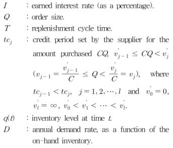
: capital opportunity cost (as a percentage).I
: earned interest rate (as a percentage).Q
: order size.T
: replenishment cycle time. : credit period set by the supplier for the amount purchased
CQ
, ′ ≤
′ (
′
≤
′
), where
, ⋯ and
′ ,
′ ∞,
′ ′ ⋯ ′.
q
(t
) : inventory level at timet
.D
: annual demand rate, as a function of the on-hand inventory.In this paper, we will concentrate on the situation in which the customer's demand rate is of a polynomial function of the following form:
, and , (1)where is the scale parameter and is the shape parameter. Given this demand function, the inventory level as a function of time will decrease rapidly initially, since the quantity demanded will be greater at a high level of inventory. As the inventory is depleted, the quantity demanded will decrease, resulting in the inventory level decreasing more slowly. Figure 1 illustrates the time behavior of the inventory level and we can interpret the slope of the curve at any point as the negative of demand rate
0 T 2T time
Figure 1. Inventory level(q(t)) vs. Time(t).
Inventory level
Q
, (2)
. (3)
Equation (3) is the differential equation and as stated by Baker and Urban[9], the mathematical expression of the inventory level over time can be determined by solving equation (3) as follows:
, (4)
, (5)
. (6)
When
t
= 0,q
(t
) =Q
. Therefore,
and
. Solving forq
(t
), we get
. (7)
Note that due to the inventory carying costs, it is clearly optimal to let the inventory level reach zero before reordering, i.e.,
q
(T
) = 0. So given thatq
(T
)= 0,
, (8)
. (9)
The purpose of this paper is to find the retailer's optimal order quantity which maximizes his annual net profit,
. For the formulation of
, we consider the inequality, ≤
. Using equation (9),the inequality can be changed to
≤
. (10)Then,
consists of the following five elements.(1) Annual sales revenue
:
=
=
. (2) Annual purchasing cost
:
=
=
.(3) Annual ordering cost
:
=
=
.(4) Annual inventory carrying cost
:
=
,
=
.(5) Annual capital opportunity cost
for ≤
:(i) Case 1(
≤
): (see Figure 2. (a)) As products are sold, the sales revenue is used to earn interest with annual rateI
during the credit period. And the number of products in stock earning interest during time is
and the
(i) Case 1(
≤
): (see Figure 2. (a)) As products are sold, the sales revenue is used to earn interest with annual rate I during the credit period . And the number of products in stock earning interest during time is
and the interest earned per order becomes
. When the credit is settled, the products still in stock have to be financed with annual rate R. Since the number of products in stock paying interest during time
becomes0 T time 0 T time
(a) ≤ (b)
Figure 2. Credit period() vs. Replenishment cycle time(
T
) Q Inventory level
Inventory level Q
interest earned per order becomes
. When the credit is settled, the products still in stock have to be financed with annual rateR
. Since the number of products in stock paying interest during time
becomes
and the interest payable per order can be expressed as
. Then
=
=
-
+
.(ii) Case 2(
): (see Figure 2. (b)) For the case of
, all the sales revenue is used to earn interest with annual rateI
during the credit period . The number of products in stock earning interest during time is
. And the number of products in stock paying interest becomes
. Therefore,
=
.Then, the annual net profit
can be expressed as
=
Depending on the relative size of
toQ
,
has two different expressions as follows:1. Case 1 (
≤
)
=
-
-
-
for ≤
, ⋯ , (11)2. Case 2 (
)
=
-
-
for ≤
, ⋯ . (12)3. Determination of Optimal Policy
The problem is to find an optimal order quantity
which maximizes
. Note that from equations (11) and (12), the annual net profit,
, and ⋯ , has the following relation:
=
at
for ⋯ .(13) It implies that the annual net profit function is continuous at
. Now, we investigate the characteristics of
. The first order condition with respect toQ
is:
=
+
+
-
+
, (14)
=
+
+
. (15)
Similarly the second order condition with respect to
Q
is:
=
-
-
+
-
+
, (16)
=
-
. (17)
For the normal condition (
≥
) as stated by Goyal [3], it can be shown that
is a concave function ofQ
and let
be the maximum value of
, respectively. While the objective function can be differentiated, the resulting equations (14) and (15) are mathematically intractable; that is, they are difficult to solve the first derivative(set equal to zero) forQ
. Therefore,
which is the maximum value of
will not be obtained in explicit form. But fortunately,
can be easily determined by using the bisection method. And then we have the following useful properties.Property 1. For ⋯ , if
≥
, then
≥
, which implies that
is increasing inQ
over
.Proof. Since
≥
,
≥ at
. It means that
≥ at
because
at
. Therefore, based on the fact that
, and ⋯ is a concave function of
Q
and
is continuous at
,
over
, which implies that
is increasing inQ
over
.Q.E.D.
Property 2. For ⋯ , if
, then
, which implies that
is decreasing inQ
over
≥
.Proof. Since
,
at
.It means that
at
because
at
. Therefore, based on the fact that
, and ⋯ is a concave function of
Q
and
is continuous at
,
over
≥
, which implies that
is decreasing inQ
over
≥
.Q.E.D.
Property 3. For any
Q
where
≥
,
, ⋯ .Proof. For
≥
, we can show that
, ⋯ , and it implies that the annual net profit function is an increasing function of . Therefore
holds since .
Q.E.D.
Property 4. For any
Q
,
, ⋯ .
Proof. From equation (13), we can show that
, ⋯ , and it implies that the annual net profit function is an increasing function of . Therefore
holds since .
Q.E.D.
Property 3 implies that
is strictly increasing for any fixed value ofQ
,
≥
asj
increases. Also, Property 4 indicates that
are strictly increasing for any fixed value ofQ
asj
increases.From the above properties, we can make the following observations about the characteristics of the annual net profit function for
Q
, ≤
, ⋯ . These observations simplify our search process to find an optimal value
.Observation 1. Let
a
be the largest index such that
andb
be the index such that ≤
. And also letm
be the maximum value ofa
andb
. Then ifk
be the largest index such that
≥ for ⋯ , then
≥ .Proof. For ⋯ ,
≤ becausea
is the largest index such that
. By Property 3,
is an increasing function of, ⋯ for
≥
. And since
≥ , we have the following relation; ≥
for
≤ (18)≥
⋯
≥
.Therefore,
≥ .Q.E.D.
Observation 2. Let
n
be the smallest index such that
. Ifk
be the largest index such that
≥ for ⋯ , then
≥ .Proof. For ⋯ ,
≥ becausen
is the smallest index such that
. By Property 4,
is an increasing function of , ⋯ for any
Q
. And since
≥ , we have the following relation; ≥
for
≤ (19)≥
⋯
≥
.Therefore,
≥ .Q.E.D.
Based on the above results, we develop the following solution procedure to determine an optimal order quantity
.Solution algorithm
Step 1. Find the largest index
a
such that ≤
and find the indexb
such that ≤
. Let
.Step 2. Find the smallest index
n
such that
.Step 3. (for the indices ⋯ ) In case
3.1 ≤
, then compute the annual net profit with equation (11) for
and go to Step 4.3.2 ≤
, then compute the annual net profit with equation (11) for
and go to Step 4.3.3
, then compute the annual net profit with equation (11) for
. Set and repeat Step 3.
Step 4. (for the indices ⋯ ) In case
4.1 ≤
, then compute the annual net profit with equation (12) for
and go to Step 5.4.2 ≤
, then compute the annual net profit with equation (12) for
and go to Step 5.4.3
, then compute the annual net profit with equation (12) for
. Set and repeat Step 4.
Step 5. (for the indices ⋯ ) In case
5.1 ≤
, in case5.1.1 ≤
, then compute the annual net profit with equation (12) for
. 5.1.2 ≤
, then compute the annualnet profit with equation (12) for
. 5.1.3
, then compute the annual netprofit with equation (12) for
. 5.2 ≤
, in case5.2.1 ≤
, then compute the annual net profit with equation (11) for
. 5.2.2 ≤
and
≥
, thencompute the annual net profit with equation (11) for
.5.2.3 ≤
, then compute the annual net profit with equation (12) for
.5.2.4
, then compute the annual net profit with equation (12) for
. 5.3
, in case5.3.1 ≤
, then compute the annual net profit with equation (11) for
. 5.3.2 ≤
, then compute theannual net profit with equation (11) for
.5.3.3
, then compute the annual net profit with equation (11) for
. Step 6. Select the optimal order quantity with the maximum annual net profit value evaluated in previous steps.4. Numerical example
To illustrate the proposed model and the solution algorithm, the following example problem is considered:
(1)
C
= $50 per unit,P
= $65 per unit,S
= $250 per order,H
= $15 per unit per year,R
= 15%,I
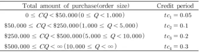
= 10%, = 1,500 and = 0.3.Table 1. Supplier's credit period schedule
Total amount of purchase(order size) Credit period
≤ ≤
≤ ≤
≤ ≤
≤ ∞ ≤ ∞
In order to solve the problem, a computer program written in QBASIC was developed to find an optimal solution as follows;
Step 1. Since
,
,
and
≥ , . And since ≤
, .Therefore,
. Step 2. Since
, .Step 3. Since
, compute by equation (11). And since ≤
, compute
by equation (11) and go to Step 4.Step 4. Since , go to Step 5.
Step 5. Since
and
≥ , compute by equation (11). And since
≤
and
≥ , compute by equation (11). Go to Step 6.
Step 6. Since = 116,593.8,
= 165,267.1,
= 180,313.4 and = 189,894.6, an optimal order quantity becomes 10,000 with its maximum annual net profit $189,894.6.As a result, the solution procedure generates an optimal solution to this problem given by:
Optimal order quantity () = 10,000 units;
Maximum annual net profit () = $189,894.6.
Following the solution algorithm, the candidate values of the optimal order quantity are
, and for and ⋯ and the optimal solution of the example appears at the credit period break quantity, . Sometimes the optimal order quantity would appear at
and we can find an example easily. For example, letS
= $150 per order andH
= $10 per unit per year(the others are same.). Then, we can find an optimal order quantity at
(= 13,186) with its maximum annual net profit $212,941.5. Conclusions
This paper dealt with the problem of the retailer's optimal order quantity determination problem when the supplier allows a delay in payments to the retailers and the length of delay in payments is a function of the retailer's order size in order to stimulate the demand for the product they produce.
Recognizing that for certain commodities, the customer's demand rate may depend on the size of the quantity on hand, we expressed the customer's demand rate of the product with a polynomial function of the on-hand inventory. The on-hand inventory level is one of the important factors related to the variation of the customer's demand rate and it is, therefore, likely to have an effect of increasing the size of each order. For the system presented, a mathematical model was developed.
After formulating the mathematical model, we developed a solution procedure that leads to identifying a retailer's optimal order quantity. To illustrate the validity of the solution procedure, an example problem was chosen and solved. The result showed that the retailer's annual net profit could be increased through a wise selection of the order size and they are consistent with our expectations.
6. References
[1] D. Mehta, The formulation of credit policy models, Management Science 15 (1968) B30-50.
[2] D.R. Fewings, A credit limit decision model for inventory floor planning and other extended trade credit arrangement, Decision Science 23 (1992) 200-220.
[3] S.K. Goyal, Economic order quantity under conditions of permissible delay in payments, Journal of the Operational Research Society 36 (1985) 335-338.
[4] K.J. Chung, A theorem on the determination of economic order quantity under conditions of permissible delay in payments, Computers and Operations Research 25 (1998) 49-52.
[5] J.T. Teng, On the economic order quantity under conditions of permissible delay in payments, Journal of the Operational Research Society 53 (2002) 915-918.
[6] Y.F. Huang, Optimal retailer's replenishment policy for the EPQ model under the supplier's trade credit policy, Production Planning & Control: The management of Operations 15 (2004) 27-33.
[7] J.T. Teng, C.T. Chang, M.S. Chern, Y.L. Chan, Retailer's optimal ordering policies with trade credit financing, International Journal of Systems Science 38 (2007) 269-278.
[8] R.I. Levin, C.P. Mclaughlin, R.P. Lamone, J.F. Kottas, Production/Operations Management: Contemporary Policy for Managing Operating Systems, McGraw-Hill, New York, 1972.
[9] R.C. Baker, T.L. Urban, A deterministic inventory system with an inventory-level-dependent demand rate, Journal of the Operational Research Society 39 (1988) 823-831.
[10] T.K. Datta, A.K. Pal, A note on an inventory model with inventory-level-dependent demand rate, Journal of the Operational Research Society 41 (1990) 971-975.
[11] P. Vrat, G. Padmanabhan, An inventory model
under inflation for stock dependent consumption rate items, Engineering Costs and Production Economics 19 (1990) 379-383.
[12] S.W.Shinn, A deterministic inventory model with an inventory-level-dependent demand rate under day-terms supplier credit in a supply chain, Journal of the Korea safety Management &
Science 11(3) (2009) 113-119.
[13] S.W. Shinn, H. Hwang, Optimal pricing and ordering policies for retailers under order-size-dependent delay in payments, Computers and Operations Research 30 (2003) 35-50.
[14] L.Y. Ouyang, C.H. Ho, C.H. Su, An optimization approach for joint pricing and ordering problem in an integrated inventory system with order-size dependent trade credit, Computers and Industrial Engineering 57 (2009) 920-930.
[15] S.W. Shinn, R. Logendran, An EOQ model for a product with stock dependent consumption rate under order-size-dependent delay in payments, Working Paper (unpublished results), School of Mechanical, Industrial and Manufacturing Engineering, Oregon State University, Corvallis, OR, U.S.A. (2011).
[16] H.C. Chang, C.H. Ho, L.Y. Ouyang, C.H. Su, The optimal pricing and ordering policy for an integrated inventory model when trade credit linked to order quantity, Applied Mathematical Modelling 33 (2009) 2978-2991.
[17] V.B. Kreng, S.J. Tan, The optimal replenishment decisions under two levels of trade credit policy depending on the order quantity, Expert Systems with Applications 37 (2010) 5514-5522.
저 자 소 개
신 성 환
현재 한라대학교 공과대학 산업 경영공학과 교수로 재직 중이며, 인하대학교 산업공학과를 졸업하 고, 한국과학기술원 산업공학과 에서 공학석사 및 공학박사학위 를 취득하였다. 주요 관심분야는 SCM, 물류관리, 생산관리 등이다.
주소: 강원도 원주시 흥업면 한라대길 28 한라대학교 공과대학 산업경영공학과