Analysis of Different 500kV HVAC Transmission Lines Lightning Shielding

Lines Lightning Shielding

Mohamed Nayel

Electrical Engineering Department, Assiut University, Assiut 71518, EGYPT

Abstract The lightning shielding of different 500 kV HVAC-TL high voltage AC transmission lines was analyzed. The studied transmission lines were horizontal flat single circuit and double circuit transmission lines. The lightning attractive areas were drawn around power conductors and shielding wires. To draw the attractive areas of the high voltage transmission lines, transmission line power conductors, shielding wires and lightning leader were modeled. Different parameters were considered such as lightningslope, ground slope and wind on lightning attractive areas. From the calculated results, the power conductors voltages affected on attractive areas around power conductors and shielding wires. For negative lightning leader, the attractive area around the transmission line power conductor increased around power conductors stressed by positives voltage and decreased around power conductors stressed by negative voltage. In spite of this, the attractivearea of the transmission line shielding wire increasedaround the shielding wire above the power conductor stressed by the positive voltage and decreased around the shielding wire above the power conductor stressed by negative voltage. The attractive areas around power conductors and shielding wires were affected by the surrounding conditions, such as lightning leader slope, ground slope. The AC voltage of the transmission lines made the shielding areas changing with time.

• Key Words : Transmission line, lightning, shielding wire, shielding failure, wind effect

*교신저자: Nayel, M.(Assiut University)

접수일 2013년 10월 31일 수정일 2013년 11월 29일 게재확정일 2013년 12월 02일

1. Introduction

Recently, the rate of building new AC high voltage transmission lines HVAC-TL’s has been increased rabidly in different developing countries such as China, Brazil, India, South Africa to transfer electrical energy from generation side locations to industrial areas. Thus, these transmission lines extended for several thousand kilometers. It was recommended that as the length of transmission lines increases as operating voltage increased. Now, several 500 kV HVAC TL has been constructed around tropical equators where there are a high lightning storm days per year. This had increased the probability of lightning strokes to the transmission lines [1-2]. To design the lightning protection strategy

of 500 kV HVAC-TL, lightning shielding failure

probability might be studied for transmission line

towers design, choice of surge arrestors and etc.. The

shielding failure occurs when the lightning leader

bypass the shielding wires and strokes the power

conductors. There are different methods have been

developed to estimate the number of the shielding

failure number. The common method to calculate the

shielding failure is electrogeometric model EGM. EGM

model is based on lightning striking distance which it

is obtained from observed lightning. Erikson had

developed the EGM to estimate the lightning shielding

failure number of transmission lines [3]. Mousa had

developed EGM to consider transmission line tower

andconductor sag in estimating lightning shielding failure numbers for transmission lines and substations [4-6].The transmission lines and substations lightning shielding design had been explained by IEEE standards [7-9]. Chowdhuri had studied the lightning striking distance based on empirical equation of the long gap voltage breakdown [10]. Rizk had estimated the striking distance from electromagnetic model of voltage condition equations for leader inception [11].

Electromagnetic model was proposed to estimate the shielding failure number directly [12-14]. Leader progress model LPM was an improvement for electromagnetic model to detect the lightning stroke to the grounded objects [15-16]. Drawing attractive areas could help in understanding shielding failure. Also it is used to check and improve the lightning shielding of transmission lines. The attractive areas around transmission lines were drawn by using EGM model [17] or by using electromagnetic model [18]. Using EGM to draw the attractive zones was limited to the attractive distance equation parameters, current and the grounded object height. The electromagnetic model could consider different conditions directly in drawing in the attractive areas around the transmission lines.

The lightning shielding and shielding failure areas around different 500 kV HVAC-TL’s were studied.

The studied TL’s are single circuit flat horizontal transmission line and double circuit transmission line.

An electromagnetic model isconstructed by using charge simulation method to simulate the downward lightning leader and transmission line power conductors and shielding wires.

2. Studied model

2.1 Studied transmission lines

Fig. 1 showed the geometric dimensions of the studied500 kV HVAC transmission lines. Fig. 1. (a) shows a horizontal flat single circuit 500 kV HVAC-TL.

It consists from 3 power conductors and 2 shielding

wires. The 3 power conductors are located at the same height 28 m and the distance between adjacent conductors is 12.5 m. The 2 shielding wires are located at height 37 m and the distance between the shielding wires is 10 m. The arrangement of power conductors and shielding wires results in a shielding angle 15.52

^o

. The power conductors phases arrangements are a, b and c from right to left, as shown in equation (1)

v

a

=V

m

sin(α), v

b

=V

m

sin(α+120), v

c

=V

m

sin(α+240) (1)

The calculation of attractive areas will be done when phase α=90

^o

. Fig. 1.(b) shows double circuits 500 kV HVAC-TL where the two circuits are distributed vertically. Each circuit consists from 3 power conductors at heights 28 m, 39 m and 50 m and spaced from the tower center by 8.25 m, 10 m and 7.2 m respectively. The 2 shielding wires are located at height 57 m with 9m separation distance between shielding wires. The arrangement of power conductors and shielding wires results in a shielding angles -0.48

^o

, 3.1798

^o

and -14.42

^o

from lower power conductor respectively. The power conductors phases arrangements for right circuit are a, b and c and for left circuit are a’, b’ and c‘ from top to down, as shown in equation (2):

v

a

=V

m

sin(α), v

b

=V

m

sin(α+120), v

c

=V

m

sin(α+240) v

a

’= V

m

sin(α+240), v

b

’=V

m

sin(α+120), v

c

’= V

m

sin(α)

(2)

The calculation of attractive areas will be done when phase α = 90

^o

. The power conductor for both transmission lines has an equivalent radius 450 mm and shielding wire radius is 50 mm.

2.2 Electromagnetic model

The charge decaying distribution [10] along the

stepped leader is assumed to be exponentially of

negative charge as

l s h c

s

l

e h

h

^l

ln( / )

, )

(

^\

ρ

^\

α ρ ρ

ρ = −

^−α

=

(3)

where,

s

is the charge density in C/m at the tip of leader stroke,

c

is the charge density in C/m at the cloud base, h

l

is the downward lightning leader length in m.

The downward lightning leader length h

l

is assumed to be constant and equal to 3 km and

c

/

s

=0.05. This value results to =10

^-3

. The downward lightning leader is simulated by N

l

discrete line charges along the

positive X, Y, Z directions. The charge density for n l

segment will be as follows:

) / (

) ( 1) (

l l l

l

l

l N

h n N h

hn h l

h n s

l t l

s t

e N e

h

e

^{− + − − +}

− −

=

^{α α α}

α ρ ρ

(4)

The potential of the downward lightning leader at any point in the space is expressed as:

( )

∑

=

−

=

^l

l l l l

l N n

n n

n

P P

V

1

ρ

\

(5)

where P _{n l} , P _n ^\ _l is the potential coefficient for n l

^th

discrete constant charge density and its image due to the ground effect (Appendix I).

(a) Single circuit horizontal flat 500 kV HVAC-TL tower

(b) Double circuit 500 kV HVAC-TL tower [Fig. 1] Studied transmission lines

The surface charges on the horizontal conductors of the transmission line are not uniform, due to the presence of the downward lightning leader. However, it is symmetrical around the X-Z plane. The surface charges on horizontal conductor along the positive Y direction is simulated by N

r

discrete line charges uniformly distributed around a factious coaxial cylinder extending along the horizontal conductor length and having radius equal to a fraction of the horizontal conductor radius r. To account for the nonuniform distribution of the charge along the positive Y direction, each of the discrete line charge is divided into N

a

sections, of which (N

a

-1) finite sections and a

semi-infinite section at the end. The length of n finite

sections is e

^m

(e

⁽ⁿ⁺¹⁾

-e

ⁿ

). The starting distance of

semi-infinite line charge d

s

=e

^{m (Na+1)}

, where m is a

constant and is chosen to be 1.84. In addition to

different line charges at radial and axial directions

inside the horizontal conductor, N

r

point charges are

placed at the intersection of the factious lines extension

with X-Z plane as shown in Fig.2. These point charges are recommended to increase the boundary and check points at intersections of horizontal conductor with X-Z plane, also, due to the presence of downward lightning leader in X-Zplane [18]. The assumed factious charges have unknown N

r

N

a

+N

r

charges for a transmission line conductor. Images of the simulation charges are considered with respect to the ground plane for maintaining zero potential at this plane. To satisfy the boundary conditions, boundary points are chosen on the horizontal conductor surface as shown in Fig. 3. A set of equations is formulated at a set of boundary points chosen on the horizontal conductor surface to determine these unknown charges. The number of boundary points is equal to the number of the unknown charges. The potential at each boundary point in the presence of downward leader is expressed as:

V l

V

Q P P

P

^{a a}

r

a

N

n

p p n p n

N n

sfl sfl n sfl n N

N n

fl fl n fl n

−

=

+

+ ∑ ∑

∑ = 1 = 1 = 1

ρ ρ

(6)

where P

fl n

, P

sfl n

, P

p n

are potential coefficients calculated at the boundary point (Appendix II) due to finite line charges, the semi-infinite line charges and point charges respectively, V is the horizontal

conductor voltage, V l is the voltage at the boundary point due to downward lightning leader. It is supposed that the lightning would strike the grounded horizontal conductor if there is an upward-directed leader from the surface of the object, as shown in Fig. 1. In this paper, a the main electric field of 230 kV/m, to sustain the upward streamer for a gap length of 10 m, is chosen to investigate the lightning stroke to the horizontal conductor for negative lightning leader charges [14-16].

[Fig. 2] Schematic arrangement of a transmission line stroked by the downward lightning leader.

[Fig. 3] Charge simulation of the horizontal conductor

[Fig. 4] Calculation model for attractive area.

(a) 500 kV HVAC-TL (b) 500 kV HVAC-TL double circuit

(a) Vertical lightning leader

(b) 45o slant lightning leader

(c) 15o slant ground

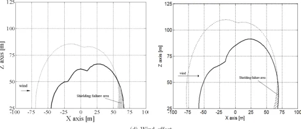
(d) Wind effect

[Fig. 5] Collection surfaces of different TL’s and different conditions by using EGM and CSM

The area around the transmission line is divided into equal d spaced mesh as shown in Fig. 4. The gap voltages around power conductors and ground wires are calculated due to locate the downward lightning leader tip at each mesh points (nd, md). Attractive area is drown by drawing a contour line of value equal to gap potential for lightning leader tip positioned at XZ directions matrix.

3. Results and discussions

Fig. 5 shows the attractive areas around power conductors and shielding wires for single and double circuits 500 kV HVAC-TLs. Fig. 5-a shows the attractive areas for vertical downward lightning leader for α=90

^o

and α=330

^o

. Flat horizontal 500 kV HVAC-TL attractive areas are less than the attractive areas around double circuit 500 kV HVAC-TL. For both studied transmission line there is no shielding failure areas. As the transmission lines power conductors voltage change as the attractive areas around power conductors change. Also the attractive area around shielding wires affected by transmission lines power conductors voltages.

Otherwise in Fig. 5-b, where the downward lightning leader has a 45

^o

slope the attractive areas of the overhead ground wires show shielding failure to the

right transmission line power conductors.

Fig. 5-c shows the effect of ground slope on the attractive areas around 500 kV HVAC-TLspower conductors and shielding wires. The ground slope decreases the attractive areas in the low side and increases the attractive areas in the high side. There is no shielding failure appears in this studied cases for both transmission lines.

Fig. 5-d shows the effect of wind on the attractive areas of both 500 kV HVAC-TLs. The wind effect is modeled by shifting the power conductors in the wind direction. So, the attractive area around the 500 kV HVAC-TL’s power conductors is shifted also in the same direction. This result to presence of the shielding failure area as the transmission lines power conductors move outside the shielding wires.

4. Conclusions

The electromagnetic model shows successfully the attractive areas around 500 kV HVAC-TL and conditions for shielding failure.The voltage of transmission line affects on striking distance. Double circuit Transmission line shielding is better than flat HVAC transmission shielding.

The attractive areas around power conductors are

affected by power conductor voltages. It is increased

around positive voltage and decreases around negative voltage. The attractive areas around transmission line shielding wire affects inversely by transmission line voltage.

The surrounding parameters (ground slope, lightning slope and wind) effects on attractive areas and may result on presenting lightning shielding failure.

REFERENCES

[1] L. Chonglin, S. Heckman, ," Using total lightning data in severe storm prediction: Global case study analysis from north America, Brazil and Australia", International Symposium on Lightning Protection (XI SIPDA), pp. 20-24, 2011.

[2] M. Nayel, Z. Jie, J. He," Analysis of AC and DC Flat Transmission Lines Lightning Shielding Failure", 7th Asia-Pacific International Conference on Lightning Crowne Plaza Chengdu, Chengdu, China, pp. 1-4, 2011.

[3] A. J. Erikson,"An improved electromagnetic model for transmission line shielding analysis", IEEE trans. on Power Delivery, Vol, 2, pp. 871-886, 1987.

[4] A. M. Mousa, K. D. Srivastava," Effect of shielding by trees on the frequency of lightning strokes to power lines", IEEE Trans. on Power Delivery, Vol.

3, pp. 724-732, 1988.

[5] A. M. Mousa, K. D. Srivastava, " The lightning performance of unshielded steel-structure transmission lines",IEEE Trans. on Power Delivery, Vol. 4, pp. 437-445, 1989.

[6] A. M. Mousa, K. D. Srivastava,"The distribution of lightning strokes to towers and along the span of shielded and unshielded power lines", Canadian Journal of Electrical and Computer Engineering, Vol. 15, pp. 115-122, 1990.

[7] IEEE Std 988-1996, IEEE guide for direct lightning stroke shielding of substations, IEEE Inc., New York, USA, 1996.

[8] IEEE Std 1243-1997, IEEE guide for improving the

lightning performance of transmission lines, IEEE Inc., New York, USA, 1997.

[9] IEEE Std 1410-1997, IEEE guide for improving the lightning performance of electric power overhead distribution lines, IEEE Inc., New York, USA, 1997.

[10] P. Chowdhuri, A. K. Kotapalli," Significant parameters in estimating the striking distance of lightning strokes to overhead lines", IEEE Trans. on Power Delivery, Vol. 4, No. 3, pp. 1970-1981, 1989.

[11] F. A. M. Rizk," Modeling of transmission line exposure to direct lightning strokes," IEEE Trans.

on Power Delivery, Vol. 5, pp. 1983-1997, 1990.

[12] J. He, Y. Tu, R. Zeng, B. Lee Jaebok, S. H. Chang, Z. Guan," Numeral Analysis Model for Shielding Failure of Transmission Line Under Lightning stroke", IEEE Trans. on Power Delivery, Vol. 20, No. 2, pp. 815-822, 2005.

[13] M. Nayel, Z. Jie, J. He, ," Significant Parameters Affecting A Lightning Stroke To A Horizontal Conductor," Journal of Electrostatics, Vol. 86, No. 5, pp. 439-444, 2010.

[14] M. Nayel, Z. Jie, J. He ,"Analysis Shielding Failure Parameters of High Voltage Direct Current Transmission Lines", Journal of Electrostatics, Vol.

70, No. 6, pp. 505-511, 2012.

[15] B. Wei, Z. Fu, H. Yuan ,"Analysis of lightning shielding failure for 500-kV overhead transmission lines based on an improved leader progression model", IEEE transactions on Power Delivery, Vol.

24, No. 3, pp. 1433-1440, 2009.

[16] B. Vahidi, M. Yahyaabadi, M. Reza Bank Tavakoli, S. M. Ahadi," Leader progression analysis model for shielding failure computation by using the charge simulation method", IEEE transactions on Power Delivery, Vol. 23, No. 23, pp. 2201-2206, 2008.

[17] N. Theethayi, Y. Liu, R. Montano, R. Thottappillil

," On the influence of conductor heights and lossy

ground in multiconductor transmission lines for

lightning interaction studies in railway overhead

traction systems", Journal of Electric Power

Systems Research, Vol. 71, No. 2, pp. 186-193, 2004.

[18] M. Nayel, "Analysis of lightning-attractive areas around high-voltage direct current transmission line", Electric Power Components and Systems, Vol.

37, pp. 146-157, 2009.

Appendixes

I- Potential coefficients for simulation downward lightning leader

The potential coefficient P n l of simulation slant finite line charge of downward lightning leader calculated at a given any point of coordinates (x

p

, y

p

, z

p

) is

⎥ ⎥

⎦

⎤

⎢ ⎢

⎣

⎡

+

+ + +

= +

EG F

G F E E E F P

_n

E

2

) (

ln 2 4

1 πε

0 l

where

( ) ( ) ( )

( ) ( )

( ) ( )

( ) ( )

(

_1`

) (

² ₁

) (

² ₁

)

²

1 2 1

1 2 1

1 2

` 1

2 1 2 2 1 2 2 1 2

l l

l

l l l

l l l

l l l

l l l l l l

n p n p n p

n n n p

n n n p

n n n p

n n n n n n

z z y y x x G

z z z z

y y y y

x x x x F

z z y y x x E

− +

− +

−

=

−

− +

−

− +

−

−

=

− +

− +

−

=

where x _{n l} ¹ , y _{n l} ¹ , z _{n l} ¹ _, x _{n l 2} , y _{n l 2} , z _{n l 2 are the} coordinates of the beginning and end of the n

^th

finite simulation line charge which has a charge density

n

,.

II- Potential coefficients for simulation horizontal conductor

a) The potential coefficient P

p

of the simulation point charges of grounded horizontal conductor calculated at a given boundary point of coordinates (x

p

, y

p

, z

p

) is

⎥ ⎥

⎦

⎤

⎢ ⎢

⎣

⎡ −

=

ni p nc p n

p

D D

P 1 1

4 1

πε

0

,

where D

pc

is the distance between the point charge and the boundary point and D

pi

is the distance between image of the point charge and the boundary point.

0

is the permittivity of free space.

b) the potential coefficient P

fl

of simulation finite line charge of grounded horizontal conductor calculated at a given boundary point of coordinates (x

p

, y

p

, z

p

) is

( )

( ) ( )

( )

( )

( ) ( )

( ) ⎥ ⎥

⎦

⎤

⎢ ⎢

⎣

⎡

+ +

+ + +

− +

−

⎥ ⎥

⎦

⎤

⎢ ⎢

⎣

⎡

+ +

+ + +

− +

= −

4 2

4 1 3 2

3 1

2 2

2 1 1 1

1 2 0

4 ln 1

δ γ δ

γ

δ γ δ

γ πε

p n fl

p n fl p

n fl

p n fl

p n fl

p n fl p n fl

p n fl n

fl

y y

y y y y

y y

y y

y y y y

y P y

where

( ) ( ) ( )

( ) ( ) ( )

( ) ( ) ( )

( ) ( ) ( )

( ) ( ) ( )

( ) ( ) ( )

( ) ( ) ( )

( ) (

2 2

) (

²

)

²

4

2 2

1 2 3

2 1 2

3 2

2 2

2 2 3

2 2

2 2 2

2 2

1 2 1

2 2

1 2 2

2 2 2

1 2

n fl p p n fl n fl p

n fl p p n fl n fl p

n fl p p n fl n fl p

n fl p p n fl n fl p

n fl p p n fl n fl p

n fl p p n fl n fl p

n fl p p n fl n fl p

n fl p p n fl n fl p

z z y y x x

z z y y x x

z z y y x x

z z y y x x

z z y y x x

z z y y x x

z z y y x x

z z y y x x

+ + + +

−

=

+ +

− +

−

=

+ + + +

−

=

+ +

− +

−

=

− + + +

−

=

− +

− +

−

=

− + + +

−

=

− +

− +

−

=

δ δ γ γ δ δ γ γ

Where y

fl n1

, y

fl n2

are the y coordinates of the beginning and end of the nth finite simulation line charge which has a charge density

fl n

, x

fl n

, z

fl n

are the X- and Z- coordinates of the n

^th

finite line charge.

c) The potential coefficient P

sfl

of simulation semi finite line charge of grounded horizontal conductor calculated at a given boundary point of coordinates (x

p

, y

p

, z

p

) is

( )

( ) ( )

( ) ⎥ ⎥

⎦

⎤

⎢ ⎢

⎣

⎡

+

− + + +

− +

= +

2 2 1

1 0

4 ln 1

β α β

α

πε

_{sfln p}

p n sfl p

n sfl

p n sfl n

sfl

y y

y y y y

y P y

where

( ) ( ) ( )

( ) ( ) ( )

( ) (

²

) (

²

)

²

2

2 2

1 2

2 2

2 1

n sfl p p n sfl n sfl p

n sfl p p n sfl n sfl p

n sfl p p n sfl n sfl p

z z y y x x

z z y y x x

z z y y x x

+ + + +

−

=

− +

− +

−

=

− + + +

−

=

α

β

α

( ) (

²

) (

²

)

²

2

= x

p

− x

sfln

+ y

sfln

− y

p

+ z

p

+ z

sfln

β

where x

sfl n

, y

sfl n

, z

sfl n

are the x-, y-, and z- coordinates of the starting point of the nth semi finite simulation line charge which has a charge density

sfl n

.

저자소개

Mohamed Nayel

․1996: Assiut University, Assiut, Egypt (BEng)

․1999: Assiut University, Assiut, Egypt (Msc(Eng))

․2004 :Eng. from Doshisha University, Japan (Ph.D)

․E-Mail : [email protected]

<Research Interest>: Power Electronics, Power

Distribution