A statistical quality control for the dispersion matrix

A statistical quality control for the dispersion matrix ^†

Jinnam Jo ¹

1 Department of Statistics and Information Science, Dongduk Women’s University

Received 30 June 2015, revised 17 July 2015, accepted 20 July 2015

Abstract

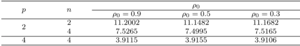
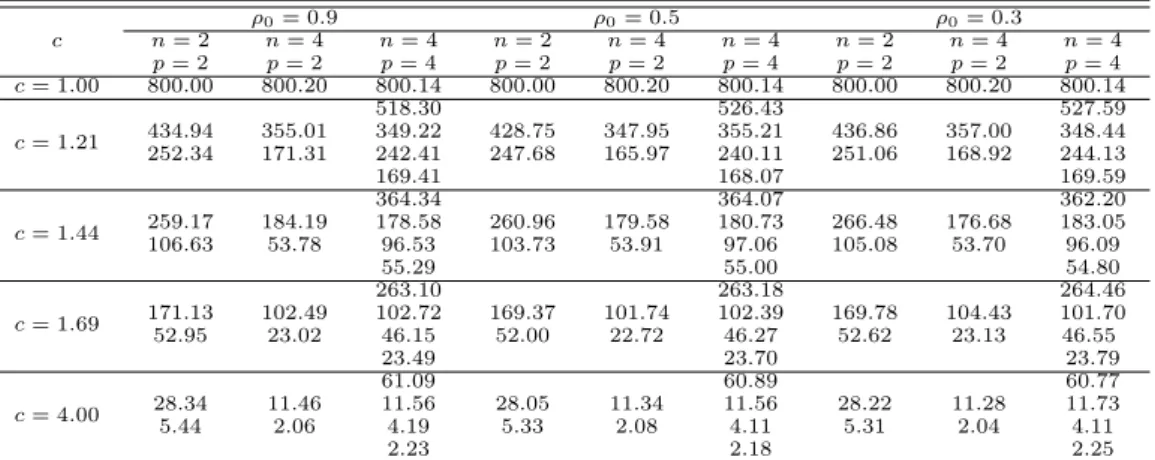
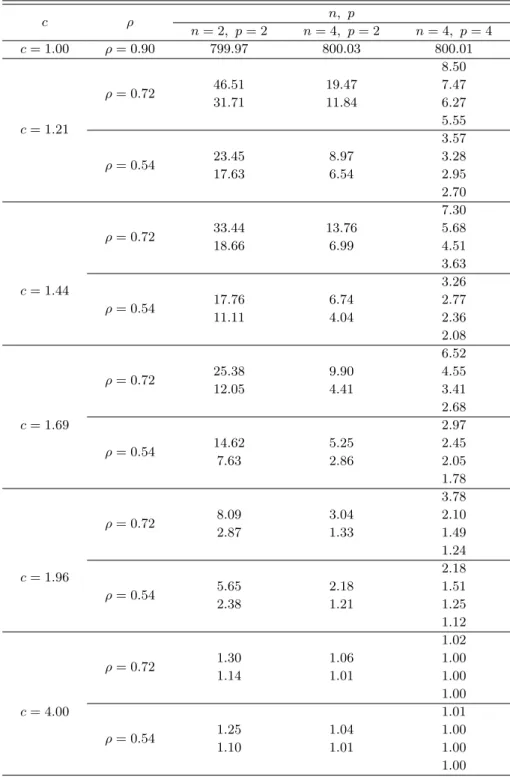
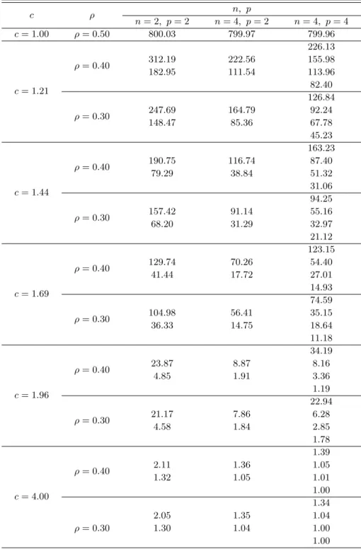
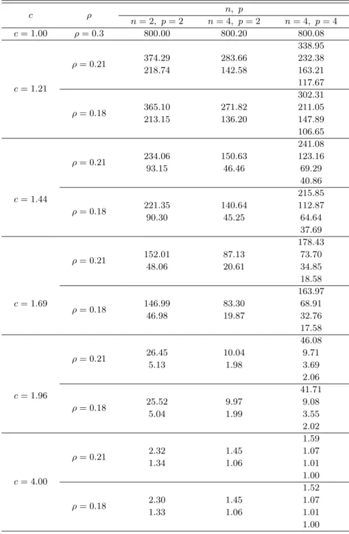
A control chart is very useful in monitoring various production process. There are many situations in which the simultaneous control of two or more related quality vari- ables is necessary. When the joint distribution of the process variables is multivariate normal, multivariate Shewhart control charts using the function of the maximum likeli- hood estimator for monitoring the dispersion matrix are considered for the simultaneous monitoring of the dispersion matrix. The performances of the multivariate Shewhart control charts based on the proposed control statistic are evaluated in term of average run length (ARL). The performance is investigated in three cases, where the variances, covariances, and variances and covariances are changed respectively. The numerical re- sults show that the performances of the proposed multivariate Shewhart control charts are not better than the control charts using the trace of the covariance matrix in the Jeong and Cho (2012) in terms of the ARLs.

Keywords: Average run length, dispersion matrix, maximum likelihood estimator, mul- tivariate Shewhart control chart.

1. Introduction

Recently there has been a growing interest in multivariate statistical process control. The multivariate control charts for monitoring the mean vector has already been studied in depth.

However, very little attention has been paid to monitor the dispersion matrix. There are various approaches to constructing control charts for multivarite data. The original work in multivariate control charts was introduced by Hotelling (1947) which is the multivariate Shewhart chart based on Hotelling’s T ² statistic. Jackson (1959), and Ghare and Torgerson (1968) presented multivariate Shewhart control charts based on Hotelling’s T ² statistic.

Other multivariate Shewhart control charts are discussed at Alt (1984), Wierda (1994), and Lowry and Montgomery (1995). Simultaneously monitoring the means and variances in the production processes in the univariate case was studied by Im and Cho (2009). The multivariate control charts for monitoring dispersion matrix were studied by Chang and Shin (2009), Aparisi et al. (2009), Na et al. (2010), Jeong and Cho (2012). In this paper, we study multivariate Shewhart control charts using the function of the maximum likelihood estimator for monitoring the dispersion matrix.

† This research was supported by the Dongduk Women’s University Grant 2013.

1

Professor, Department of Statistics and Information Science, Dongduk Women’s University, Seoul 136-

714, Korea. E-mail: [email protected]

2. Notation and assumptions

It will be convenient to let σ represent the vector of standard deviations of the p variables in the multivariate normal distribution of the observation. According to the notation in Jeong and cho (2012), let µ 0 , Σ 0 , and σ 0 be the in-control values of µ, Σ, and σ. And we assume that the in-control parameter values are known. Suppose that we take a sample of n ≥ 1 independent observation vectors at each sampling point, where the sampling points are d time units apart. Let X kij be the jth observation for variable i at sampling point k for k = 1, 2, · · · , i = 1, 2, · · · , p and j = 1, 2, · · · , n, and let the corresponding standardized observation be

Z _kij = (X _kij − µ 0i )/σ _0i ,

where µ _0i is the ith component of µ ₀ and σ _0i is the ith component of σ ₀ . Also let Z kj = (Z k1j , Z k2j , · · · , Z kpj )

, j = 1, 2, · · · , n

be the vector of standardized observations for the jth observation at sampling point k. Let Σ Z be the covariance matrix of Z kj , and let Σ Z0 be the in-control value of Σ Z . The in-control distribution of Z kij is standard normal, so Σ Z0 is also the in-control correlation matrix of the unstandardized observations.

Let ¯ X ki = P n

j=1 X kij /n be the sample mean for variable i at sampling point k, and define the standardized sample mean to be

Z ki = √

n( ¯ X ki − µ 0i )/σ 0i , i = 1, 2, · · · , p.

When n ≥ p, some control statistics used for monitoring Σ are functions of the sample estimates b Σ _Z . At sampling point k, let b Σ _Z

be the maximum likelihood estimator of Σ _Z , where the (i, i

) element of b Σ _Z

is P n

j=1 Z _kij Z _ki

_j /n.

We investigate a number of multivariate Shewhart control charts for Simultaneously mon- itoring the dispersion matrix.

3. Multivariate Shewhart control charts

We will discussmultivariate Shewhart control charts based on the statistic L _k proposed by Hui (1980) which use the sample generalized variances for monitoring the process dispersion matrix

L _k = |b Σ _k |

|Σ 0 | , (3.1)

where Σ 0 is known. It is known that the distribution of √

n(L k − 1) is asymptotically normal with mean 0 and variance 2p (Anderson, 1958). But, we can not get the exact distribution.

Because of using small sample size in the control chart study, we need to calculate control

limits and ARLs by using simulations. When sample size n is large, the approximate expected

value of L _k is 1 and the variance of L _k is 2np.

For large sample size n, the approximate three-sigma control limits for L _k for monitoring Σ are then

UCL = 1 + 3 p 2np, LCL = 1 − 3 p

2np.

For a Shewhart control chart, control limits based on the statistic L k would be set by using percentage point of L k , and signals whenever

L _k > h, (3.2)

where h can be obtained to satisfy a specified in-control ARL.

If the process shifts from Σ ₀ then it is difficult to obtain the exact distribution of L _k . Thus it is necessary to use simulations in order to obtain the percentage points of L _k when the process is out-of-control state.

In this paper, we evaluated the performance of the control charts based on the average run length performance. The ARLs for the multivariate control chart byusing (3.1) when the process is in control can be obtained by using 10,000 replications.

In our computation, each control chart was calibrated so that the on-target ARL was approximately equal to 800.0 and the sample size for each control chart was n ≥ p for p = 2 and p = 4. The performance of the control charts for monitoring the dispersion matrix depends on the value of Σ. The following types of shifts were considered;

(1) variances are changed and covariances are not changed, (2) covariances are changed and variances are not changed, (3) variances and covariances are simultaneously changed.

The control limits h and ARLs for multivariate Shewhart control charts based on the generalized variances are obtained by using 10,000 replications. Table 3.1 gives the values of h for n ≥ p for p = 2, 4 and ρ = 0.9, 0.5, 0.3 when the ARL is approximately 800.

Table 3.1 Values of h for multivariate Shewhart control charts for various values of p and ρ when the in-control ARL is approximately 800

p n ρ

ρ

= 0.9 ρ

= 0.5 ρ

= 0.3

2 2 11.2002 11.1482 11.1682

4 7.5265 7.4995 7.5165

4 4 3.9115 3.9155 3.9106

4. Numerical performances and concluding remarks

The multivariate Shewhart control charts with control statistic given by (3.1) are compared on the basis of their ARLs. The ARLs of multivariate control chart when the process is in- control are fixed to be 800.

Table 4.1 gives p ARLs in each cell when one, two, · · · , p variances are changed and covariances are not changed respectively. Here standard deviations are changed from σ 0 to σ = √

cσ 0 , for c = 1.21, 1.44, 1.69, 4.00. Table 4.1 shows that the performances of the control

charts for the three different correlations are very similar.

Table 4.2 gives ARLs for n = 2, 4, p = 2, 4 and three different in-control correlation coefficients ρ ₀ = 0.9, 0.5, 0.3 when covariances are changed and variances are not changed.

Table 4.2 shows that the performances of the control charts for the larger ρ 0 = 0.9 are better than the other cases.

As shown in Tables 4.1-4.2, the multivariate Shewhart control charts for monitoring the dispersion matrix are effective in detecting changes in Σ. In case of larger ρ 0 = 0.9, mul- tivariate Shewhart control charts are very effective in detecting changes in covariances in Σ.

For n = 2, 4 and p = 2, 4, Tables 4.3-4.5 give p ARLs in each cell when one, two, · · · , p vari- ances and p covariances are simultaneously changed, respectively. Here standard deviations are changed from σ 0 to σ = √

cσ 0 for c = 1.21, 1.44, 1.69, 4.00, and covariances are changed from ρ ₀ = 0.9 to ρ = 0.72, 0.54, ρ ₀ = 0.5 to ρ = 0.4, 0, 3, and ρ ₀ = 0.3 to ρ = 0.21, 0.18.

As shown in Tables 4.3-4.5, the multivariate Shewhart control charts for monitoring the dispersion matrix are also effective in detecting simultaneously changes in variances and covariances in Σ. In case of larger ρ ₀ = 0.9, this chart is very effective in detecting changes in variances and covariances in Σ.

From Tables 4.1-4.5, the performances of the multivariate Shewhart control charts using the function of the maximum likelihood estimator for monitoring the dispersion matrix are not better than the control charts using the trace of the covariance matrix in the Jeong and Cho (2012) in terms of the ARLs.

Table 4.1 ARL when variances are changed and covariances are not changed c

ρ

= 0.9 ρ

= 0.5 ρ

= 0.3

n = 2 n = 4 n = 4 n = 2 n = 4 n = 4 n = 2 n = 4 n = 4

p = 2 p = 2 p = 4 p = 2 p = 2 p = 4 p = 2 p = 2 p = 4

c = 1.00 800.00 800.20 800.14 800.00 800.20 800.14 800.00 800.20 800.14 c = 1.21 434.94 355.01

518.30

428.75 347.95

526.43

436.86 357.00

527.59

349.22 355.21 348.44

252.34 171.31 242.41 247.68 165.97 240.11 251.06 168.92 244.13

169.41 168.07 169.59

c = 1.44 259.17 184.19

364.34

260.96 179.58

364.07

266.48 176.68

362.20

178.58 180.73 183.05

106.63 53.78 96.53 103.73 53.91 97.06 105.08 53.70 96.09

55.29 55.00 54.80

c = 1.69 171.13 102.49

263.10

169.37 101.74

263.18

169.78 104.43

264.46

102.72 102.39 101.70

52.95 23.02 46.15 52.00 22.72 46.27 52.62 23.13 46.55

23.49 23.70 23.79

c = 4.00 28.34 11.46

61.09

28.05 11.34

60.89

28.22 11.28

60.77

11.56 11.56 11.73

5.44 2.06 4.19 5.33 2.08 4.11 5.31 2.04 4.11

2.23 2.18 2.25

Table 4.2 ARL when covariances are changed and variances are not changed

ρ

ρ

= 0.9 ρ

= 0.5 ρ

= 0.3

n = 2 n = 4 n = 4 ρ n = 2 n = 4 n = 4 ρ n = 2 n = 4 n = 4

p = 2 p = 2 p = 4 p = 2 p = 2 p = 4 p = 2 p = 2 p = 4

ρ = 0.90 799.97 800.03 800.01 ρ = 0.50 800.03 799.97 799.96 ρ = 0.30 800.02 799.99 799.91

ρ = 0.81 146.47 80.10 32.10 ρ = 0.45 650.22 98.11 492.97 ρ = 0.27 754.77 726.30 675.02

ρ = 0.72 66.71 30.88 10.20 ρ = 0.40 546.44 85.64 324.78 ρ = 0.24 712.12 684.26 580.62

ρ = 0.63 42.60 17.91 5.55 ρ = 0.35 482.88 13.08 236.18 ρ = 0.21 673.64 648.89 505.60

ρ = 0.54 32.09 12.75 4.00 ρ = 0.30 427.37 340.48 176.18 ρ = 0.18 647.71 601.97 454.94

ρ = 0.45 26.13 10.33 3.14 ρ = 0.25 393.80 301.41 142.38 ρ = 0.15 629.76 572.04 417.92

ρ = 0.36 22.64 8.77 2.72 ρ = 0.20 368.00 271.00 118.91 ρ = 0.12 623.18 560.71 379.24

ρ = 0.27 20.71 7.81 2.49 ρ = 0.15 347.88 259.82 103.05 ρ = 0.09 698.08 551.83 347.75

ρ = 0.18 19.51 7.38 2.30 ρ = 0.10 339.78 246.03 94.04 ρ = 0.06 586.08 540.54 334.35

ρ = 0.09 18.77 6.93 2.22 ρ = 0.05 331.25 239.92 89.36 ρ = 0.03 570.05 520.34 324.06

Table 4.3 ARL when variances and covariances are changed (ρ

= 0.9)

c ρ n, p

n = 2, p = 2 n = 4, p = 2 n = 4, p = 4

c = 1.00 ρ = 0.90 799.97 800.03 800.01

c = 1.21

ρ = 0.72 46.51 19.47

8.50 7.47

31.71 11.84 6.27

5.55

ρ = 0.54 23.45 8.97

3.57 3.28

17.63 6.54 2.95

2.70

c = 1.44

ρ = 0.72 33.44 13.76

7.30 5.68

18.66 6.99 4.51

3.63

ρ = 0.54 17.76 6.74

3.26 2.77

11.11 4.04 2.36

2.08

c = 1.69

ρ = 0.72 25.38 9.90

6.52 4.55

12.05 4.41 3.41

2.68

ρ = 0.54 14.62 5.25

2.97 2.45

7.63 2.86 2.05

1.78

c = 1.96

ρ = 0.72 8.09 3.04

3.78 2.10

2.87 1.33 1.49

1.24

ρ = 0.54 5.65 2.18

2.18 1.51

2.38 1.21 1.25

1.12

c = 4.00

ρ = 0.72 1.30 1.06

1.02 1.00

1.14 1.01 1.00

1.00

ρ = 0.54 1.25 1.04

1.01 1.00

1.10 1.01 1.00

1.00

Table 4.4 ARLs when variances and covariances are changed (ρ

= 0.5)

c ρ n, p

n = 2, p = 2 n = 4, p = 2 n = 4, p = 4

c = 1.00 ρ = 0.50 800.03 799.97 799.96

c = 1.21

ρ = 0.40 312.19 222.56

226.13 155.98

182.95 111.54 113.96

82.40

ρ = 0.30 247.69 164.79

126.84 92.24

148.47 85.36 67.78

45.23

c = 1.44

ρ = 0.40 190.75 116.74

163.23 87.40

79.29 38.84 51.32

31.06

ρ = 0.30 157.42 91.14

94.25 55.16

68.20 31.29 32.97

21.12

c = 1.69

ρ = 0.40 129.74 70.26

123.15 54.40

41.44 17.72 27.01

14.93

ρ = 0.30 104.98 56.41

74.59 35.15

36.33 14.75 18.64

11.18

c = 1.96

ρ = 0.40 23.87 8.87

34.19 8.16

4.85 1.91 3.36

1.19

ρ = 0.30 21.17 7.86

22.94 6.28

4.58 1.84 2.85

1.78

c = 4.00

ρ = 0.40 2.11 1.36

1.39 1.05

1.32 1.05 1.01

1.00

ρ = 0.30

2.05 1.35

1.34 1.04

1.30 1.04 1.00

1.00

Table 4.5 ARLs when variances and covariances are changed (ρ

= 0.3)

c ρ n, p

n = 2, p = 2 n = 4, p = 2 n = 4, p = 4

c = 1.00 ρ = 0.3 800.00 800.20 800.08

c = 1.21

ρ = 0.21 374.29 283.66

338.95 232.38

218.74 142.58 163.21

117.67

ρ = 0.18 365.10 271.82

302.31 211.05

213.15 136.20 147.89

106.65

c = 1.44

ρ = 0.21 234.06 150.63

241.08 123.16

93.15 46.46 69.29

40.86

ρ = 0.18 221.35 140.64

215.85 112.87

90.30 45.25 64.64

37.69

c = 1.69

ρ = 0.21 152.01 87.13

178.43 73.70

48.06 20.61 34.85

18.58

ρ = 0.18 146.99 83.30

163.97 68.91

46.98 19.87 32.76

17.58

c = 1.96

ρ = 0.21 26.45 10.04

46.08 9.71

5.13 1.98 3.69

2.06

ρ = 0.18 25.52 9.97

41.71 9.08

5.04 1.99 3.55

2.02

c = 4.00

ρ = 0.21 2.32 1.45

1.59 1.07

1.34 1.06 1.01

1.00

ρ = 0.18 2.30 1.45

1.52 1.07

1.33 1.06 1.01

1.00

References

Alt, F. B. (1984). Multivariate control charts. In Encyclopedia of Statistical Sciences, edited by S. Kotz and N. L. Johnson, John Wiley, New York.

Anderson, T. W. (1958). An introduction to multivariate statistical analysis, Wiley, New York.

Aparisi, F., Jabaioyes, J. and Carrion, A. (2009). Statistical properties of the |S| multivariate control chart.

Communications in Statistics-theory and methods, 28, 2671-2686.

Chang, D. J. and Shin, J. K. (2009). Variable sampling interval control charts for variance-covariance matrix.

Journal of the Korean Data & Information Science Society, 21, 999-1008.

Ghare, P. H. and Torgerson, P. E. (1968). The multicharacteristic control chart. Journal of Industrial Engineering, 19, 269-272.

Hotelling, H. (1947). Multivariate quality control, techniques of statistical analysis, McGraw-Hill, New York, 111-184.

Hui, Y. V. (1980). Topics in statistical process control, Ph. D. Thesis, Virginia Politechnic Institute and State University, Blacksberg, Virginia.

Im, C. D. and Cho, G. Y. (2009). Multiparameter CUSUM charts with variable sampling intervals. Journal of the Korean Data & Information Science Society, 20, 593-599.

Jackson, J. S. (1959). Quality control methods for several related variables. Technometrics, 1, 359-377.

Jeong, J. I. and Cho, G. Y. (2012). Multivariate Shewhart control charts for monitoring the variance- covariance matrix. Journal of the Korean Data & Information Science Society, 23, 617-628.

Lowry, C. A. and Montgomery, D. C. (1995). A review of multivariate control charts. IIE Transactions, 27, 800-810.

Na, O., Ko, B. and Lee, S. (2010). Cusum of squares test for discretely observed sample from multidimen- sional diffusion processes. Journal of the Korean Data & Information Science Society, 21, 555-560.

Wierda, S. J. (1994). Multivariate statistical process control - recent results and directions for future re-

search. Statistica Neerlandica, 48, 147-168.