©Copyrights 2012. The Korean Academy of Conservative Dentistry. 245
This is an Open Access article distributed under the terms of the Creative Commons Attribution Non-Commercial License (http://creativecommons.org/licenses/
by-nc/3.0) which permits unrestricted non-commercial use, distribution, and reproduction in any medium, provided the original work is properly cited.
1) Features of samples from normal populations
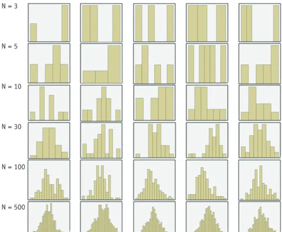
Various parametric tests make assumptions of the normal distribution, including t-test, analysis of variance (ANOVA), correlation, and regression. Different from some researcher’s understanding, tests of normality are not for the normality of observed data but for normality of the population distribution of a random characteristic; e.g. assuming normality for the population distribution of the characteristic is reasonable when referring to the observed sample data. Actual distribution of the characteristic in a random sample chosen from a population with normal distribution doesn’t appear normal, especially when the sample size is small (Figure 1). Distributions of larger samples tend to resemble the distribution of the characteristic in the population better by taking on a bell-shaped curve when the values of a characteristic in the population are plotted against their frequency.
Open lecture on statistics
ISSN 2234-7658 (print) / ISSN 2234-7666 (online) http://dx.doi.org/10.5395/rde.2012.37.4.245
Statistical notes for clinical researchers: assessing normal distribution (1)
Figure 1. Histograms of a characteristic of interest in various sizes of random samples from a normal population (N = 10,000) with a normal distribution (sample size = 3, 5, 10, 30, 100 and 500).
N = 3
N = 5
N = 10
N = 30
N = 100
N = 500
Hae-Young Kim
Department of Dental Laboratory Science & Engineering, Korea University College of Health Science, Seoul, Korea
*Correspondence to Hae-Young Kim, PhD, DDS Associate Professor, Department of Dental Laboratory Science &
Engineering, Korea University College of Health Science, San 1 Jeongneung 3-dong, Seongbuk-gu, Seoul, Korea 136-703 TEL, +82-2-940-2845; FAX, +82-2-909-3502, E-mail, [email protected]
246 www.rde.ac
2) Testing of the normality using SPSS statistical package
Using the SPSS output you can find out several methods to test normality of the data.
In SPSS you can find information needed for normality tests under the following menu:
Analysis – Descriptive Statistics – Explore
(1) Eyeball test
• You can look at a histogram of your data and see whether the distribution of the sample resembles a normal distribution or not; e.g., whether the histogram looks like a bell-shape or not? Is the shape symmetrical or not? Or you can chose a Q-Q (“Q” stands for quantile) plot to see whether all the data points have a linear tendency and lie on the diagonal or not.
Mean = 100.8097 Std. Dev. – 21.7292 N = 100
Histogram Normal Q-Q plot of Y
Frequency Expected normal
20
15
10
5
0
4
2
0
-2
-4
60.00 80.00 100.00 120.00 40.00 40 60 80 100 120 140 160
Y Observed value
Kim HY
http://dx.doi.org/10.5395/rde.2012.37.4.245
247 www.rde.ac
• Most statistical packages provide both types of graphs. The advantage of the eyeball test is its easiness and simplicity and the disadvantage is that the criteria for determination are not clear.
• Furthermore confusion arises from the fact that samples from a normal population don’t necessarily show a normal distribution; few samples look like normal distributions, especially samples with small size, as we can see in Figure 1.
Therefore this eyeball test may be more meaningful in relatively large samples (e.g., n > 50).
(2) Shapiro-Wilk test & Kolmogorov-Smirnov test
• Generally formal normality tests such as the Shapiro-Wilk test or the Kolmogorov-Smirnov test have been well known.
Those tests assess a null hypothesis that distribution of the data is normal. The Shapiro-Wilk test has been reported to be more powerful than the Kolmogorov-Smirnov test in testing normality (Razali et al., 2011).
3) Problems of formal normality tests
There are problems in formal normality tests that the probability of rejecting the null hypothesis of normality tends to slightly increase as sample size increases: for large samples (n > 300), these formal normality tests may be unreliable.
Following example shows incompatible results in normality test for a large sample (n = 500). While the data seems to be approximately normal by an eyeball test, the Shapiro-Wilk test and Kolmogorov-Smirnov test give an opposite conclusion that the distribution of the data may be different from normality (p < 0.05).
Tests of normality
Kolmogorov-Smirmova Shapiro-Wilk
Statistic df Sig. Statistic df Sig.
Y 0.076 100 0.167 0.983 100 0.216
a, Lilliefors significance correct.
Mean = 99.9127 Std. Dev = 19.72003 N = 500
Histogram Normal Q-Q plot of Y
Frequency Expected normal
60 50 40 30 20 10 0
3 2 1 0 -1 -2 -3
40.00 60.00 80.00 100.00 120.00 140.00 20 40 60 80 100 120 140 160
Y Observed value
http://dx.doi.org/10.5395/rde.2012.37.4.245
248 www.rde.ac
Though methods above provide useful information, still it is not easy to determine whether the example data may satisfy the assumption of normal distribution or not. Confusion may arise because they suggest incompatible conclusions as shown above. More helpful methods to determine normality can be discussed at the next statistical note.
Reference
1. Razali NM, Wah YB. Power comparisons of Shapiro-Wilk, Kolmogorov-Smirnov, Lilliefors and Anserson-Darling tests. J Stat Model Anal 2011;22:21-33.
Tests of normality
Kolmogorov-Smirmova Shapiro-Wilk
Statistic df Sig. Statistic df Sig.
Y 0.044 500 0.020 0.993 500 0.029
a, Lilliefors significance correct.
Kim HY
http://dx.doi.org/10.5395/rde.2012.37.4.245