A Review on the Analysis of Life Data Based on Bayesian Method: 2000~2016

베이지안 기법에 기반한 수명자료 분석에 관한 문헌 연구 : 2000~2016

원동연¹․임준형¹․심현수¹․성시일²․임헌상³․김용수^4†

1경기대학교 일반대학원 산업경영공학과, ²인제대학교 산업경영공학과

3삼성전자 품질보증실, ⁴경기대학교 산업경영공학과

A Review on the Analysis of Life Data Based on Bayesian Method: 2000~2016

Dong-Yeon Won¹․Jun Hyoung Lim¹․Hyun Su Sim¹․Si-il Sung² Heonsang Lim³․Yong Soo Kim^4†

1Dept. of Industrial and Management Engineering, Kyonggi University Graduate School

2Dept. of Industrial and Management Engineering, Inje University

3Division of Quality Assurance, Samsung Electronics

4Dept. of Industrial and Management Engineering, Kyonggi University

Purpose: The purpose of this study is to arrange the life data analysis literatures based on the

Methods: The Bayesian method produces a more accurate estimates of other traditional methods

Results: In many studies, there are comparisons of estimation methods for the Bayesian method

Conclusion: To verify the characteristics of the Bayesian method which are more superior to

Also, comparative study is required by various distributions, thereby providing guidelines necessary.

1)

Keywords: Bayesian Method, Life Data, Sample Size, MCMC(Markov chain Monte Carlo),

* 본 연구는 2017학년도 경기대학교 대학원 연구원장학생 장학금 지원에 의하여 수행되었음.

†교신저자 [email protected]

2017년 7월 31일 접수; 2017년 8월 22일 수정본 접수; 2017년 9월 1일 게재 확정.

1. 서 론

시스템의 고장은 인명 및 재산 피해를 초래하므로 이를 예방하기 위해 일반적인 품질 관점이 아닌 신뢰 성 관점에서 관리되어야 한다. 또한, 과학기술 발전에 따른 시스템의 첨단화 및 복잡화로 다양한 산업에서 높은 수준의 신뢰성이 요구되고 있다.

신뢰성을 평가하기 위한 다양한 방법론 가운데 수 명자료를 활용한 방법은 먼저 시스템의 수명 관측 값 을 가장 잘 설명할 수 있는 적합 수명분포를 선정하고 정확한 모수를 추정한다. 여기서 참모수에 가까운 통 계 값을 추정하는 것은 매우 중요하며 부정확한 추정 은 무의미한 분석 결과를 도출해 명확한 신뢰성 평가 가 이뤄질 수 없다.

일반적으로 사용되는 수명분포의 모수 추정방법에 는 전통적 기법인 최소제곱추정법(least square estima- tion, LSE)과 최대우도추정법(maximum likelihood es- timation, MLE)이 있다. 전통적 기법은 충분한 표본크 기에서 참모수와 근사한 추정 값을 제공하나, 표본의 크기가 작아질수록 추정 정확도가 낮아진다는 단점 을 가지고 있다[1]. 이러한 이유로 충분한 표본 확보 가 어려운 산업에서는 전통적 기법을 대체할 추정기 법이 필요하며 그 대안으로 추정에 더 적은 오차를 보 이는 베이지안 방법을 기대할 수 있다[1].

베이즈 정리는 1763년 이항분포의 모수를 추론하는 문제로 처음 등장했으며, 라플라스 등 여러 수학자에 의해 재발견되고 발전됨으로써 다양한 문제에 응용이 시도될 수 있는 발판이 만들어졌다. 그러나 다양한 이 론적 심화발전에도 불구하고 연산에서 발생하는 막대 한 시간적 비용으로 현실적 문제 해결에 활용되지 못한 다는 학문적 한계를 보였다. 20세기 말 시작된 정보화 시대에서 하드웨어 및 소프트웨어의 발달은 이러한 문 제점을 해결하여 복잡한 계산을 쉽게 연산할 수 있도록 하였으며, 이는 다양한 산업에서 베이지안 방법을 활 용하고 응용 연구가 진행되는 등 범용성이 증가하도록 기여하고 방법론의 영향력은 점차 확대되었다[2-7].

여러 산업계의 높은 관심에도 불구하고, 수명자료분 석에 관한 베이지안 방법의 문헌연구는 [8]과 같은 정 성적인 리뷰가 대부분이었으며 정량적인 방법으로 정 리한 문헌연구는 이루어지지 않고 있다. 따라서, 본 연 구는 베이지안 방법에 관해 세 가지 분류 기준을 통하 여 정량적 문헌 분석을 제공하고자 한다. 이 문헌연구

의 구성은 다음과 같다. 먼저 제 2장에서는 문헌 분류기 준으로 선택한 베이지안 방법의 핵심적인 세 가지 특성 을 소개하며, 각각은 크게 표본크기, 시뮬레이션 알고리 즘, 사전정보의 유무 및 정확성으로 구성된다. 제 3장 에서는 앞서 제시한 분류기준을 중심으로 2000년 이후 발표된 38편의 논문을 분류하였다. 마지막으로 제 4장에 서는 기대효과 및 향후 연구방향을 제시하고자 한다.

2. 베이지안을 활용한 수명자료 분석 문헌의 분류기준과 설명

본 장에서는 베이지안 방법의 세 가지 특성을 고려 한 문헌의 분류기준을 제안한다. 먼저, 베이지안 방법 의 가장 큰 특성은 작은 표본에서 전통적 방법과 비교 하여 추정 정확성이 우수하다는 것이다. 그러나 관련 문헌자료에서 작은 표본에 대한 기준을 명확히 제시 하지 않고 있어 사용자가 실제 활용 시 어려움을 야기 할 수 있다. 따라서, 첫 번째 문헌 분류기준으로 표본 크기를 선택하여 관련 문헌에서 다룬 표본크기에 대 해 파악하고자 한다. 두 번째 분류기준은 베이지안 방 법에 활용되는 알고리즘의 종류로 정의하였다. 베이 지안 추정량은 조건부 사후분포로 이루어져 있어 단 순한 방법으로는 연산이 어렵다는 한계가 존재하며 이를 해결하기 위해 다양한 알고리즘이 적용된다. 그 중 대표적으로 사용하는 세 가지 방법으로 문헌을 구 분하였다. 마지막으로 사전정보의 적절성에 따라 베 이지안 방법의 결과에 영향을 미치는 특성을 반영하 여 이를 분류기준으로 선정하였다.

2.1 표본크기

모집단의 특성을 파악하기 위한 전수조사는 매우 이

상적이나 현실적으로 어려워 표본조사가 일반적으로

이루어진다. 또한, 표본조사로부터 얻어진 데이터를

통해 참 값에 가까운 근사 값을 얻는 것은 매우 중요하

다. 베이지안 방법을 활용하여 수명자료를 분석한 문

헌의 대부분은 베이지안 방법과 다른 기법간의 정확성

을 비교하며, 이의 결과는 표본크기에 따라 다양한 형

태를 보인다. 일반적으로 관련문헌의 연구는 최대우

도추정법과 추정 정확성을 비교하고 결론으로 표본크

기 등 조건에 따른 적합한 추정 방법을 가이드라인으로

제시한다. 최대우도추정법이란 확률밀도함수(Probability

density function) 또는 확률질량함수(Probability mass function)로부터 독립된 관측 값이 주어질 때, 우도함수 (Likelihood function)를 최대화시킴으로써 선택된 분포 하에서 관측된 표본과의 일치를 최대화시키는 모수 값 을 선택하는 방법론이다. 많은 문헌들의 연구결과에서 최대우도추정법은 표본크기가 클 경우 모수에 대한 높 은 추정 정확도를 제공하지만, 그 크기가 작을 경우 적 절한 사전정보가 있는 베이지안 방법보다 추정 정확도 가 떨어진다는 것을 알 수 있다[9, 10]. 이는 최대우도추 정법과 같이 우도함수를 활용하는 베이지안 방법에서 적절한 사전정보의 역할이 표본크기가 작은 환경에서 모수에 대한 추정 정확성을 높여준다고 할 수 있다. 따 라서, 충분한 표본 확보가 어려운 경우, 더 우수한 신뢰 성 평가가 이루어질 수 있다.

2.2 시뮬레이션 알고리즘

베이즈 정리란 이전의 경험과 현재의 증거를 토대 로 어떤 사건의 확률을 추론하는 것으로

개의 사건

__ ⋯_

가 표본공간

를 배타적으로 분할하 고 먼저 발생한 사건

가 표본공간의 임의의 사건일 경우, 그 후에 발생될 특정 사건

가 발생할 확률은 식 (1)과 같이 쓰일 수 있으며 연속확률분포를 활용하 여 표본

가 주어졌을 때 모수

일 확률을 표현한 사 후분포의 형태로 나타내면 식 (2)와 같다.

^_{ }





_^⋅^_

^^⋅^



^^{   }

(1)





(2)

식 (2)에서 좌변

는 사후(posterior)분포이고, 우변은 사전(prior) 정보

와 발생 가능한 모든 사 건을 고려한 우도(Likelihood)함수

로 표현되 며 분모는 상수로서 주변분포이자 증거라고 불린다.

앞서 서론에서는 베이지안 방법을 이용하는 것에 대하여 제약이 존재한다는 것을 언급하였다. 베이지 안 방법이 어려운 이유는 모수가 2개 이상인 경우 주 변분포를 연산하기 위한 적분 계산이 복잡하기 때문

이다. 이를 해결하기 위해서는 다양한 방법이 존재하며 그 중 마르코프 체인 몬테카를로(Markov chain Monte Carlo, MCMC)가 가장 대표적 방법이다. MCMC란 마 코프 연쇄와 몬테카를로 적분을 이용하여 적분 값을 사후분포로부터 독립적으로 샘플링하며 이러한 과정 을 단계적으로 반복 수행하고 궁극적으로 이를 통해 목표한 분포의 기댓 값 및 특성을 근사적으로 도출해 내는 베이지안 추론방법이다. MCMC의 장점은 사후 분포로부터 마르코프 체인을 통해 표본을 얻어내며 많은 반복을 통해 사후분포를 모사하여 적분을 하지 않아도 모수를 추정할 수 있다는 것이다. 최근 문헌연구 에서는 베이즈 추정량을 연산하기 위해 MCMC뿐만 아니라 Lindley’s approximation도 많이 사용하고 있다.

따라서, 본 절에서는 MCMC의 알고리즘인 Metropolis- Hastings와 Gibbs sampling, 그리고 Lindley’s approxi- mation의 알고리즘에 대해 살펴보고자 한다.

2.2.1 Metropolis-Hastings

MCMC의 반복시행은 임의의 초기 값에서 확률보행 (random walk)의 형태로 진행되며, MCMC 중 Metro- polis-Hastings알고리즘이 널리 적용된다. 수행과정에 서는 커널이라고도 불리는 임의의 제안분포(proposal distribution)가 필요하며 임의의 제안분포와 제안된 동작 중 일부를 거부하는 방법을 사용하여 확률보행 을 생성한다. 특히, 위 알고리즘은 같은 MCMC 중 다 른 하나인 Gibbs sampling보다 빠른 연산을 수행한다 는 장점이 있으나 반대로 수식이 고차원일수록 느려 져 상대적으로 매우 비효율적이다. 마코프 연쇄는 임 의의 제안분포

와 불변하는 사후분포

를 가 정하거나 이용하여 등식을 성립시키는 채택확률

를 포함한 식 (3)으로 표현가능하다.

^ _{ }^^ _^^^{ }^_{ }^^ 

(3) 위의 식 (3)을 통해 채택확률을 도출할 수 있으며 이를 이용한 Metropolis-Hastings 알고리즘은 다음과 같다.

Algorithm:

Step 1: 임의의 모수인 변수

를 선정하고 알고리즘 을 시작한다(

).

Step 2: 현재 변수는

, 제안된 모수는 제안분포로부 터 생성해

로 표현한다.

Step 3: 다음과 같이 채택확률

를 구한다.

  





^ _^^

^_{ }^^ ^





Step 4: 균일분포(0, 1)로부터

를 생성한다.

Step 5:

이면

을, 그 외에는

를 채택하여

_{ }

로 사용한다.

Step 6:

를

증가시킨다.

Step 7: Step 2로 돌아가 Steps 2-6을 충분히 반복 수행 한다.

2.2.1 Gibbs sampling

MCMC에서 Metropolis-Hastings 다음으로 많이 다 뤄지는 Gibbs sampling은 결합확률보다 조건부확률 로부터 샘플링이 쉬운 경우 유용하게 사용된다. 일반 적으로 고차원의 랜덤 변수를 가지는 결합확률은 구 하기 힘들고, 이를 통한 난수발생은 더 어려운 문제 다. 이 같은 문제를 해결할 수 있는 통계적 기법이 바 로 Gibbs sampling이다[11]. 각 변수의 조건부확률로 부터 랜덤표본을 반복적으로 생성하면 적절한 조건 하에서 이들의 극한분포가 결합확률이 된다는 사실 에 근거하여 모수를 추정해 최종적으로 기댓 값 및 특 성을 도출할 수 있다[8]. 이 알고리즘은 결합확률 또 는 그와 연관된 계산을 근사하기 위해 주로 사용되며, Metropolis-Hastings 알고리즘의 특별한 경우로서 일반 적인 적용에는 제약이 있지만

차원의 랜덤변수를



개의 1차원변수로 가정함으로써 고차원의 영역에 서 빠르고 난수 추출이 단순하므로 쉽게 사용된다. 다 음은 결합확률

을 구하기 위한 Gibbs sampling의 알고리즘이다.

Algorithm:

Step 1: 확률변수

에 임의의 초기 값을 할 당하고

라 표현한다.

Step 2:

로부터 난수발 생 후,

에 할당한다.

Step 3: 순차적으로

까지 조건부분포

 ≠ 

로부터 난수를 발생시킨다.

Step 4:

를

증가시킨다.

Step 5: Step 2로 돌아가 Steps 2-4를 충분히

번 반복 수행한다.

Step 6:

를

증가시킨다.

Step 7: 얻어진

개의 랜덤표본을 이용하여

⋯ _

을 근사한다.

2.2.3 Lindley’s Approximationb

베이즈 추정량을 연산하기 위해 MCMC 이외에도 Lindley’s approximation라는 접근법이 종종 활용된다.

Lindley’s approximation은 표본이 충분히 클 경우 다 음 식 (4)와 같은 분석적으로 해결 불가능한 적분간의 비를 구하여 모수를 추정함으로써 많은 저자들에 의 해 다양한 분포의 베이지안 추정량을 구하기 위한 접 근법으로 사용되었다[12].

 









(4) 이는 테일러 시리즈를 확장해 적분을 표현한 것으 로 정보적 사전분포와 무정보적 사전분포의 구분 없 이 시뮬레이션 실행 시, MCMC 대비 전반적으로 적 은 변동성을 갖는다는 장점을 보인다[13].

2.3 사전정보의 유무 및 정확성

추론을 위한 베이지안 방법에서 사전정보가 합리 적으로 선택될 경우 사후분포는 명확하게 추정될 수 있으며 결과적으로 우수한 기댓 값을 계산할 수 있다.

그러나 제반 여건으로 인해 정확한 사전정보를 알아 내는 것은 쉬운 일이 아니며 많은 경우에서 객관성을 가지는 전형적인 무정보적(non-informative) 사전분포 를 이용한다[14].

사전정보의 선정은 매우 중요하며 동시에 어려운 문

제이다. 베이지안 방법에서 사전정보는 필수요소로서

모수에 대한 주어진 정보나 믿음이 없는 경우 무정보

적 사전분포를 사용한다. 무정보적 사전분포는 상대

적으로 결과에 민감하지 않은 균등분포와 제프리 사전

분포가 많이 활용된다. 균등분포는 수학자 라플라스

에 의해 널리 이용되어 왔으며 제프리 사전분포는 제

프리가 피셔정보를 사용하여 사전확률의 영향력을 최

대한으로 줄인 사전분포이다. 무정보적 사전분포와는

반대로 자료에 기반하여 사전정보를 구하고 추론에 사

용하고자 할 때, 과거자료나 연산자의 주관적인 믿음

Author Year Method Sample Size

MLE Bayesian ≤10 ≤25 ≤50 over 50

Taheri and Behboodian[15] 2001 O 5

Akama[5] 2002 O 46

Singh et al.[16] 2002 O O 5 20

Assoudou and Essebbar[17] 2003 O O 21 61

Nassar and Eissa[18] 2005 O O 15 30, 50

Guikema[19] 2005 O 1~10 10~20

Jaheen[20] 2005 O O 5, 8 12

Soliman et al.[21] 2006 O O 19

Huang et al.[22] 2006 O 5

Gebraeel and Lawley[23] 2008 O 25

Singh et al.[10] 2008 O O 10 20 30, 40

Kundu[24] 2008 O O 20 30

Amin[25] 2008 O 25

Soliman[26] 2008 O O 20 50 100

Kundu and Gupta[27] 2008 O O 15, 23, 25 50 75

Ahmed et al.[1] 2010 O O 25 50 100

Kundu and Howlader[28] 2010 O O 20, 25, 40

Wang et al.[29] 2011 O 8

Kim et al.[30] 2011 O O 20 30, 50

Ahmed and Ibrahim[31] 2011 O O 25 50 100

Seo and Park[3] 2011 O 72

Jaheen and Al Harbi[32] 2011 O O 15, 50, 40 60

Li et al.[33] 2011 O 30

Guure et al.[34] 2012 O O 25 50 100

Fu et al.[35] 2012 O 12, 17, 20 100

Guure and Ibrahim[36] 2012 O O 25 50 100

Huang and Wu[12] 2012 O O 19, 20

Ahmed et al.[37] 2012 O O 25, 50 100

Kundu and Raqab[38] 2012 O 25, 50

Lin et al.[6] 2013 O 46

Mun et al.[9] 2013 O O 5

Son[39] 2013 O O 15 30 100

Jang and Lee[4] 2013 O O 77

Ahmed[40] 2014 O O 25 50 100

Hao and Su[41] 2014 O 16

Achcar et al.[42] 2015 O O 5 25 50

Cho et al.[43] 2016 O O 3, 5, 7, 10 15, 20, 25 30

Table 1 Classification of Group A based on sample size and estimation method

이 내재된 정보적 사전분포를 이용할 수 있다. 그러나

주관적인 견해가 포함되었기 때문에 적합하지 않은 사 전정보에 의하여 구하고자 하는 값을 정확히 얻지 못 하게 될 수 있다. 본 연구에서는 베이지안 방법의 기존 문헌에 기반하여 정보적 사전분포 및 무정보적 사전분 포의 사용여부를 확인하고 분류해보고자 한다.

3. 베이지안 문헌의 분류

본 장에서는 총 38편의 문헌을 제 2장에서 제시한

문헌의 분류기준을 토대로 적절한 추가고려사항까지

반영하여 <Table 1>~<Table 3>과 같이 정리한다. 각

표의 정리 대상은 해당하는 분류기준과 추가고려사

Author Year Probability Distribution Data Type

MCMC Lindley’s approximation Metropolis-

Hastings

Gibbs sampler Nassar and Eissa[18] 2005 Exponentiated Weibull complete, type 2 O

Guikema[20] 2005 BurrtypeXII complete O

Singh et al.[10] 2008 Generalized Exponential complete O

Kundu[24] 2008 Weibull progressive type 2 O O

Amin[25] 2008 Pareto progressive type 2 O

Kundu and Gupta[27] 2008 Generalized Exponential complete O O

Ahmadi et al.[44] 2009 BurrtypeXII, Exponential,

Pareto, Weibull(1-par) complete O

Kundu and Howlader[28] 2010 Inverse-Weibull type 2 O

Seo and Park[3] 2011 Logistic complete O

Jaheen and Al Harbi[32] 2011 Exponentiated Weibull type 2 O O

Guure et al.[34] 2012 Weibull complete O

Guure and Ibrahim[36] 2012 Weibull type 2 O

Huang and Wu[12] 2012 Weibull progressive type 2 O

Ahmed et al.[37] 2012 Weibull type 1 O

Kundu and Raqab[38] 2012 Weibull type 2 O

Lin et al.[6] 2013 Log-normal, Weibull type 1 O

Son[39] 2013 Pareto(2-par) complete O

Ahmed[40] 2014 Weibull interval O O

Hao and Su[41] 2014 Inverse-Gausian complete O

Achcar et al.[42] 2015 Exponential(2-par) complete O

Cho et al.[43] 2016 Weibull complete O

Table 2 Classification of Group B based on simulation algorithm, distribution and data type

항을 만족하는 그룹 A, B, C로 재구성되었으며 다수

문헌이 중복된다. 그룹 A는 표본의 크기 외에 추정 방 법이 함께 고려되어 분류가능하며 그룹 B는 사용된 시뮬레이션 알고리즘의 종류와 더불어 확률분포와 자료의 형태, 그룹 C는 사전정보의 형태와 확률분포 로 동시 분류가능하다.

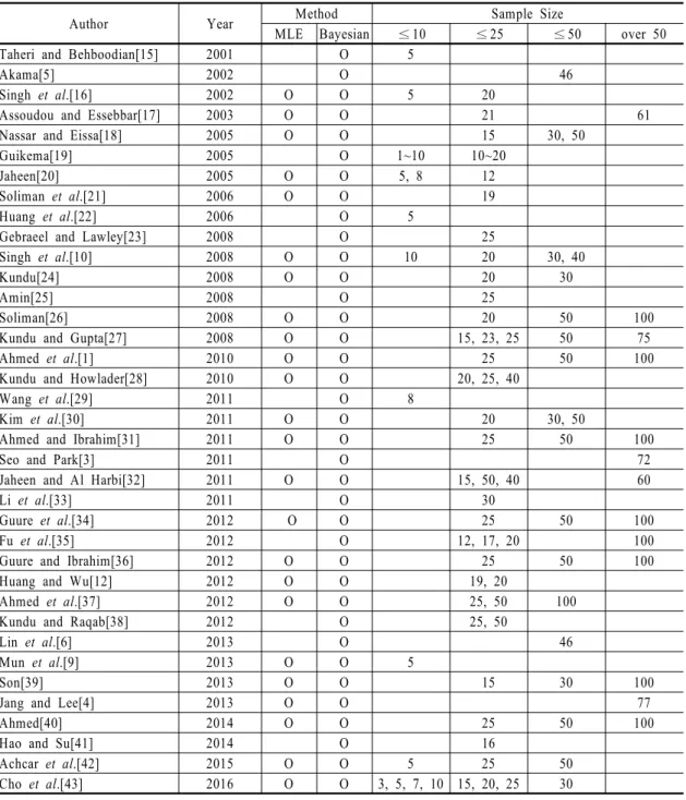
먼저 <Table 1>은 표본의 크기에 따라 그룹 A를 분 류한 것으로, 분석결과 약 65%의 문헌이 베이지안 방 법과 최대우도추정법의 정확도를 비교하고 있음을

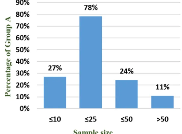
<Fig. 1>을 통해 확인 가능하다. 표본의 크기에 따른 사용 비율은 <Fig. 2>와 같으며, 시뮬레이션에 쓰이는 표본의 크기는 10 초과 25 이하에 약 78%로 가장 많 이 분포되어있고 더 작은 크기인 10 이하는 약 27%로 많이 다루어지고 있지 않다. 또, 62%의 문헌이 보다 쉬운 식별을 위해 5배수의 표본만을 사용하는 경향을 보였다.

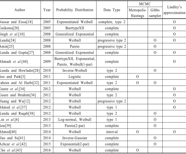
<Table 2>는 시뮬레이션 알고리즘에 따라 그룹 B 를 분류하여 분석한 결과로, 사용된 확률분포의 종 류와 비율은 <Fig. 3>과 같이 정리되며 약 62%의 다 수문헌에서 확률분포로 와이블분포 또는 확장형태 의 와이블분포 등을 사용하고 있다는 사실을 알 수 있다. 즉, 수명자료는 일반적으로 와이블분포를 가 정한다. 그 외에도 지수, 버-타입 XII, 파레토, 로지스 틱 등 다양한 확률분포가 적용되었다. 수명자료의 유형으로는 절반가량이 완전자료였으며 중단자료 의 경우 <Fig. 4>와 같이 세부적으로 살펴볼 수 있다.

정시중단과 구간중단은 약 18%와 9%로 매우 적게 사

용되었고 그 외에는 정수중단과 점진형 정수중단이

나타났다. 또 <Fig. 5>에서 방법론은 MCMC와 Lindley’s

approximation 모두 유사하게 적용되고 있음을 알 수

있으며, 복수로 사용된 경우의 수도 약 14%로 확인

가능하다.

Fig. 1 Comparative study to MLE in Group A Fig. 2 Sample size in Group A

Fig. 3 Probability distribution in Group B Fig. 4 Censored data’s type in Group B

Fig. 5 Simulation algorithm in Group B

Author Year Probability Distribution

Prior

Informative Non-Informative Exact Wrong Distribution

Taheri and Behboodian[15] 2001 Binorminal Uniform

Guikema[19] 2005 Weibull O Gausian Uniform

Jaheen[20] 2005 BurrtypeXII O Gamma

Soliman et al.[21] 2006 Weibull O Gamma

Huang et al.[22] 2006 Gausian, Log-normal Jeffrey

Singh et al.[10] 2008 Generalized Exponential O Gamma

Kundu[24] 2008 Weibull O Gamma

Amin[25] 2008 Pareto O Gamma

Kundu and Gupta[27] 2008 Generalized Exponential O Gamma Ahmadi et al.[43] 2009 BurrtypeXII, Exponential,

Pareto, Weibull(1-par) O Gamma

Ahmed et al.[1] 2010 Weibull Jeffrey, extension

of Jeffrey Kundu and Howlader[28] 2010 Inverse-Weibull O Gamma

Wang et al.[29] 2011 Threshold O Gamma

Kim et al.[30] 2011 Exponentiated Weibull O Bivarate

Ahmed and Ibrahim[31] 2011 Weibull Jeffrey, extension

of Jeffrey

Seo and Park[3] 2011 Logistic O

Gausian×

Logistic×

Trianglular Jaheen and Al Harbi[32] 2011 Exponentiated Weibull O Gamma×

Gamma

Guure et al.[34] 2012 Weibull extension of Jeffrey

Fu et al.[35] 2012 Pareto Jeffrey

Guure and Ibrahim[36] 2012 Weibull O Gamma generalised

Huang and Wu[12] 2012 Weibull O Bivarate

Ahmed et al.[37] 2012 Weibull Jeffrey, extension

of Jeffrey

Kundu and Raqab[38] 2012 Weibull O Gamma

Lin et al.[6] 2013 Exponential, Log-normal O Gausian, Gamma

Mun et al.[9] 2013 Weibull O O Gamma

Jang and Lee[4] 2013 Weibull O Exponential×

Weibull

Ahmed[40] 2014 Weibull O Gamma

Hao and Su[41] 2014 Inverse-Gausian O Gausian,

Gamma

Achcar et al.[42] 2015 Exponential(2-par) O Copula, Gamma Jeffrey

Cho et al.[43] 2016 Weibull O O Gamma Jeffrey

Table 3 Classification of Group C based on prior information

× : joint.

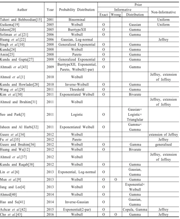
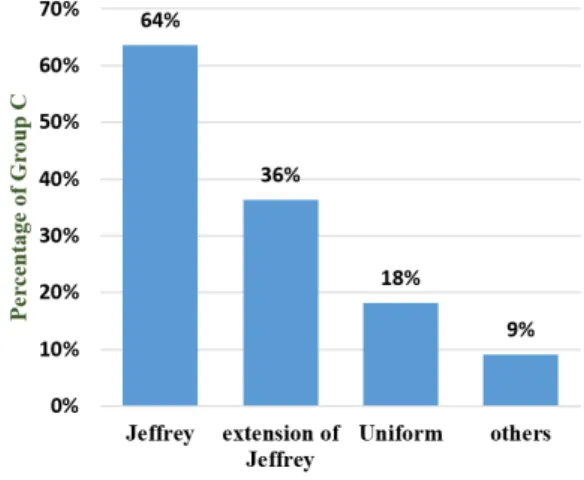
<Table 3>은 사전정보의 유무 및 정확성을 기준으 로 그룹 C를 구분하였으며, 전반적으로 문헌들은 정 보적 사전분포를 많이 사용했음을 <Fig. 8>을 통해 알 수 있다. 각 <Fig. 7>과 <Fig. 8>에 따르면, 정보적 사

전분포 하에서 감마분포의 사용률은 약 74%로 가장

높았으며 무정보적 사전분포는 제프리 사전분포, 확

장형 제프리 사전분포, 균등분포 순으로 많이 사용

됐다.

Fig. 6 Prior information in Group C

Fig. 7 Informative prior distribution’s type in Group C

Fig. 8 Non-informative prior distribution’s type in Group C

4. 결 론

본 문헌연구에서는 베이지안 방법에 기반한 2000 년대 이후 발표된 38편의 문헌을 정량적으로 분류해 표로 정리하였다. 베이지안 방법은 작은 표본에서 전 통적인 방법 대비 추정의 정확성이 높으며 추정 과정 에서 특정 알고리즘과 사전정보가 필요하다는 특징 을 가지고 있다. 따라서 문헌을 분류하는 기준으로 이 러한 베이지안 방법의 세 가지 특성을 고려한 분류기 준을 수립한 다음, 표로 정리하여 제시하였다.

결과적으로, 다수문헌에서 최대우도추정법과의 비 교를 다루고 있으며, 베이지안 방법에 기반한 대부분 의 문헌들은 10 초과 25 이하의 표본 하에서 연구가 이 루어져, 그 외의 표본 수에 대한 연구는 부족한 실정이 다. 작은 표본에서 우수성을 보이는 특성을 검증하기 위해서는 현재 부족한 10 이하의 매우 작은 표본에서 의 연구가 필요하다. 두 번째로, 수명자료에서 일반적 으로 쓰이는 와이블분포 이외에도 지수, 버-타입 XII, 파레토, 로지스틱분포 등이 다양하게 적용되었으므 로, 베이지안 방법 하에서 여러 분포에 따른 추정의 정 확도를 비교해볼 필요가 있다. 자료의 형태는 완전자 료가 절반이었으며 특히 정시중단과 구간중단자료에 대한 연구는 많이 이루어지지 않았다. 또한, 시뮬레이 션 알고리즘은 MCMC와 Lindley’s approximation 모두 고르게 사용되고 있으며, 사전정보로는 감마분포, 제 프리 사전분포, 확장형 제프리 사전분포, 균등분포가 주로 사용되었다는 사실을 알 수 있다.

References

[1] Ahmed, A. O. M., Al-Kutubi, H. S., and Ibrahim, N. A.

(2010). “Comparison of the Bayesian and maximum likelihood estimation for Weibull distribution”. Journal of Mathematics and Statistics, Vol. 6, No. 2, pp. 100-104.

[2] Kim, S. U. and Lee, K. S. (2008). “At-site Low Flow Frequency Analysis Using Bayesian MCMC: Ⅱ. Appli- cation and Comparative Studies”. Journal of Korea Water Resources Association, Vol. 41, No. 1, pp. 49-63.

[3] Seo, Y. M. and Park, K. B. (2011). “Uncertainty Analy-

sis for Parameters of Probability Distribution in Rainfall

Frequency Analysis by Bayesian MCMC and Metropo-

lis Hastings Algorithm”. Journal of Environmental Science International, Vol. 20, No. 3, pp. 329-340.

[4] Jang, B. and Lee, J. (2013). “A Study on life Prediction of Railway Safety Equipment Using Bayesian Me- thod”. Autumn Conference of the Korean Society for Railway, pp. 29-34.

[5] Akama, M. (2002). “Bayesian analysis for the results of fatigue test using full-scale models to obtain the accu- rate failure probabilities of the Shinkansen vehicle axle”.

Reliability Engineering and System Safety, Vol. 75, No.

3, pp. 321-332.

[6] Lin, J., Asplund, M., and Parida, A. (2013). “Bayesian parametric analysis for reliability study of locomotive wheels”. Reliability and Maintainability Symposium (RAMS), pp. 1-6.

[7] Song, S. R., Park, J., and Kim, Y. (2017). “Hierarchical Bayesian analysis for a forest stand volume”. Journal of the Korean Data and Information Science Society, Vol.

28, No. 1, pp. 29-37.

[8] Khatibisepehr, S., Huang, B., and Khare, S. (2013).

“Design of inferential sensors in the process industry: A review of Bayesian methods”. Journal of Process Con- trol, Vol. 23, No. 10, pp. 1575-1596.

[9] Mun, B. M., Sun, E. J., and Bae, S. J. (2013). “Bayesian Reliability Estimation for Small Sample-Sized One- shot Devices”. Journal of Applied Reliability, Vol. 13, No. 2, pp. 99-107.

[10] Singh, R., Singh, S. K., Singh, U., and Singh, G. P.

(2008). “Bayes estimator of generalized-exponential parameters under Linex loss function using Lindley’s approximation”. Journal of Data Science, Vol. 7, pp.

65-75.

[11] Lee, W. D., Lee, C. S., and Kang, S. G. (1997). “An Estimation of Parameters in Weibull Distribution using Gibbs Sampler”. Conference of the Korean Society of Industrial Information Systems, pp. 521-533.

[12] Huang, S. R. and Wu, S. J. (2012). “Bayesian estimation and prediction for Weibull model with progressive cen- soring”. Journal of Statistical Computation and Simula- tion, Vol. 82, No. 11, pp. 1607-1620.

[13] Singh, U., Singh, S. K., and Yadav, A. S. (2015). “Baye- sian Estimation for Exponentiated Gamma Distribution Under Progressive Type-II Censoring Using Different

Approximation Techniques”. Journal of Data Science, Vol. 13, No. 3, pp. 551-567.

[14] Kim, E. L. (2003). “Bayesian Change Point Analysis us- ing Gibbs Sampling in a Sequence of Multivariate Normal Observations with a Single Change Point”.

Department of Statistics Graduate School, Chonnam National University.

[15] Taheri, S. M. and Behboodian J. (2001). “A Bayesian approach to fuzzy hypotheses testing”. Fuzzy Sets and Systems, Vol. 123, No. 1, pp. 39-48.

[16] Singh, U., Gupta, P. K., and Upadhyay, S. K. (2002).

“Estimation of exponentiated Weibull shape parameters under LINEX loss function”. Communications in Stati- stics-Simulation and Computation, Vol. 31, No. 4, pp.

523-537.

[17] Assoudou, S. and Essebbar, B. (2003). “A Bayesian Model for Markov Chains via Jeffrey’s Prior”. Commu- nications in Statistics-Theory and Methods, Vol. 32, No. 11, pp. 2163-2184.

[18] Nassar, M. M. and Eissa, F. H. (2005). “Bayesian Esti- mation for the Exponentiated Weibull Model”. Com- munications in Statistics-Theory and Methods, Vol. 33, No. 10, pp. 2343-2362.

[19] Guikema, S. D. (2005). “A comparison of reliability es- timation methods for binary systems”. Reliability Engi- neering and System Safety, Vol. 87, No. 3, pp. 365-376.

[20] Jaheen, Z. F. (2005). “Estimation based on generalized order statistics from the Burr model”. Communications in Statistics-Theory and Methods, Vol. 34, No. 4, pp.

785-794.

[21] Soliman, A. A., Ellah, A. A., and Sultan, K. S. (2006).

“Comparison of estimates using record statistics from Weibull model: Bayesian and non-Bayesian approaches”.

Computational Statistics and Data Analysis, Vol. 51, No. 3, pp. 2065-2077.

[22] Huang, H. Z., Zuo, M. J., and Sun, Z. Q. (2006). “Baye- sian reliability analysis for fuzzy lifetime data”. Fuzzy Sets and Systems, Vol. 157, No. 12, pp. 1674-1686.

[23] Gebraeel, N. Z. and Lawley, M. A. (2008). “A Neural Network Degradation Model for Computing and Upda- ting Residual Life Distributions”. IEEE Transactions on Automation Science and Engineering, Vol. 5, No. 1, pp.

154-163.

[24] Kundu, D. (2008). “Bayesian Inference and Life Tes- ting Plan for the Weibull Distribution in Presence of Progressive Censoring”. Technometrics, Vol. 50, No. 2, pp. 144-154.

[25] Amin, Z. H. (2008). “Bayesian inference for the Pareto lifetime model under progressive censoring with bino- mial removals”. Journal of Applied Statistics, Vol. 35, No. 11, pp. 1203-1217.

[26] Soliman, A. A. (2008). “Estimations for Pareto model using general progressive censored data and asym- metric loss”. Communications in Statistics-Theory and Methods, Vol. 37, No. 9, pp. 1353-1370.

[27] Kundu, D. and Gupta, R. D. (2008). “Generalized ex- ponential distribution: Bayesian estimations”. Compu- tational Statistics and Data Analysis, Vol. 52, No. 4, pp.

1873-1883.

[28] Kundu, D. and Howlader, H. (2010). “Bayesian infe- rence and prediction of the inverse Weibull distribution for Type-II censored data”. Computational Statistics and Data Analysis, Vol. 54, No. 6, pp. 1547-1558.

[29] Wang, W., Carr, M., Xu, W., and Kobbacy K. (2011).

“A model for residual life prediction based on Brownian motion with an adaptive drift”. Microelectronics Reli- ability, Vol. 51, No. 2, pp. 285-293.

[30] Kim, C., Jung, J., and Chung, Y. (2011). “Bayesian esti- mation for the exponentiated Weibull model under Type II progressive censoring”. Statistical Papers, Vol.

52, No. 1, pp. 53-70.

[31] Ahmed, A. O. M. and Ibrahim, N. A. (2011). “Bayesian survival estimator for Weibull distribution with cen- sored data”. Journal of applied Sciences, Vol. 11, No. 2, pp. 393-396.

[32] Jaheen, Z. F. and Al Harbi, M. M. (2011). “Bayesian es- timation for the exponentiated Weibull model via Mar- kov chain Monte Carlo simulation”. Communications in Statistics-Simulation and Computation, Vol. 40, No.

4, pp. 532-543.

[33] Li, H., Yuan, R., Peng, W., Liu, Y., and Huang, H. Z.

(2011). “Bayesian inference of Weibull distribution based on probability encoding method”. International Conference on IEEE, pp. 365-369.

[34] Guure, C. B., Ibrahim, N. A., and Ahmed, A. O. M.

(2012). “Bayesian Estimation of Two-Parameter Weibull

Distribution Using Extension of Jeffreys’ Prior Infor- mation with Three Loss Functions”. 2012 Mathematical Problems in Engineering, pp. 1-13.

[35] Fu, J., Xu, A., and Tang, Y. (2012). “Objective Bayesian analysis of Pareto distribution under progressive Type-II censoring”. Statistics and Probability Letters, Vol. 82, No. 10, pp. 1829-1836.

[36] Guure, C. B. and Ibrahim, N. A. (2012). “Bayesian ana- lysis of the survival function and failure rate of Weibull distribution with censored data”. 2012 Mathematical Problems in Engineering, pp. 1-19.

[37] Ahmed, A. O. M., Ibrahim, N. A., Adam, M. B. and Arasan, J. (2012). “Bayesian survival and hazard esti- mate for Weibull censored time distribution”. Journal of Applied Sciences, Vol. 12, pp. 1313-1317.

[38] Kundu, D. and Raqab, M. Z. (2012). “Bayesian infe- rence and prediction of order statistics for a Type-II cen- sored Weibull distribution”. Journal of statistical plan- ning and inference, Vol. 142, No. 1, pp. 41-47.

[39] Son, Y. S. (2013), “Objective Bayesian Estimation of Two-Parameter Pareto Distribution”. Korean Journal of Applied Statistics, Vol. 26, No. 5, pp. 713-723.

[40] Ahmed, A. O. M. (2014). “Comparison of the Bayesian Methods on Interval-Censored Data for Weibull Distri- bution”. Open Journal of Statistics, Vol. 4, No. 8, pp.

570-577.

[41] Hao, H. and Su, C. (2014). “A Bayesian Framework for Reliability Assessment via Wiener Process and MCMC”.

2014 Mathematical Problems in Engineering.

[42] Achcar, J., Moala, F. and Boleta, J. (2015). “Generalized exponential distribution: A Bayesian approach using MCMC methods”. International Journal of Industrial Engineering Computations, Vol. 6, No. 1, pp. 1-14.

[43] Cho, H., Lim, J. and Kim, Y. S. (2016). “A Comparison of the Reliability Estimation Accuracy between Baye- sian Methods and Classical Methods Based on Weibull Distribution”. Journal of Korean Institute of Industrial Engineers, Vol. 42, No. 4, pp. 256-262.

[44] Ahmadi, J., Jozani, M. J., Marchand E. and Parsian A.

(2009). “Bayes estimation based on k-record data from

a general class of distributions under balanced type loss

functions”. Journal of Statistical Planning and Infe-

rence, Vol. 139, No. 3, pp. 1180-1189.