Effect of Random Poisson's Ratio on the Response Variability of Composite Plates

(1)

Variability of Composite Plates

Noh, Hyuk-Chun^† Yoon, Young-Cheol^*

···

Abstract

Together with the Young’s modulus the Poisson’s ratio is another independent material parameter that governs the behavior of a structural system. Therefore, it is meaningful to evaluate separately the influence of the parameter on the random response of the structural system. To this end, a formulation dealing with the spatial randomness in the Poisson’s ratio in laminated composite plates is proposed. The main idea of the paper is to transform the fraction form of the constitutive coefficients into the expanded form in an ascending order of the stochastic field function. To validate the adequacy of the formulation, a square plate is chosen and the computation results are compared with those obtained using conventional Monte Carlo simulation. It is observed that the results show good agreement with those by the Monte Carlo simulation(MCS).

Keywords : stochastic field function, random poisson’s ratio, coefficient of variation, response variability, taylor’s expansion

···

†책임저자, 종신회원․세종대학교 토목환경공학과 조교수

* 교신저자, 종신회원․명지전문대학 토목과 조교수 Tel: 02-300-1135 ; Fax: 02-303-1132 E-mail: [email protected]

∙이 논문에 대한 토론을 2011년 2월 28일까지 본 학회에 보내주시 면 2011년 4월호에 그 결과를 게재하겠습니다.

1. Introduction

It is an intrinsic feature of materials to have uncertainty, which is generally known as randomness, over the spatial domain. It is true not only for the isotropic-like material of structural steel but also for the complex composite material of concrete. The composite materials can also have randomness in their material properties such as the elastic modulus, shear modulus and the Poisson’s ratio. In the composite materials, the processes of lay-up and curing are relatively more complex than the conventional isotropic materials. The constitution of composites, i.e., the fibers and matrix materials, endows it with more complexity and the material uncertainties spread over the domain. The strength of the composites is also known to be affected by the fiber volume fraction (Cohen, 2001), which is random in nature. For these reasons, the possibility of spatial uncertainty in the material properties of composites is expected to be

considerably high. In this respect, the correct evaluation of the response variability in the composite materials is highly demanded.

Two main categories of the stochastic finite element static analysis are on the effects of spatial randomness of material properties and the geometrical parameters on the response variability(Choi and Noh, 2000; Deodatis and Shinozuka, 1989; Stefanou and Papadrakakis, 2004; Noh, 2004). Developments of the analysis schemes of composite structures with random material properties, however, are relatively limited. Since the mathematical expressions for composite materials is complex, which makes the formulations for the non-statistical approach difficult, the Monte Carlo simulation(MCS) approach has been employed for various stochastic problems including free vibration analysis(Singh et al., 2009). The effect of random geometrical parameters assumed as distributed in a Gaussian way has also been performed (Wang, 1990). Onkar et al.(2004, 2007), Kam et

(2)

al.(1993) and Lekou and Philippidis(2008) have demonstrated the effect of random material properties regarding the failure probability or reliability. Hilton and Yi(1999) dealt with the topic on the delamination of composites. In the case of the spectral version of the stochastic FEM methodology, N.Z. Chen(2008) suggested a methodology for laminated composite plates that assumes the elastic and shear moduli to be Gaussian random variable.

We assume that the Poisson’s ratio is only the random parameter in the system in order to investigate the sole effect of the parameter on the response variability in laminated composite structures. In case of composite materials, owing to the symmetry in the compliance matrix, a reciprocal relation exists between the material constants along mutually perpendicular material axes. Applying this feature and then employing the Taylor’s expansion on the typical fraction form of constitutive relations(up to 4^th order), we construct the constitutive matrix in the power series expansion form, which enables us to complete a formulation for stochastic finite element scheme for composite materials.

The suggested scheme is applied to an example composite plate, and the results obtained by the proposed scheme are compared with those obtained by MCS performed in this study.

2. Random material parameter

2.1 Randomness in Poisson’s ratio

If we use the generally accepted expression for random parameter, the Poisson’s ratio νcan obviously be written as follows:

( )

¹ f_ν

( )

^, Dstr

ν x =ν ⎡⎣ + x ⎤⎦ x∈ ₍₁₎

Here, we need to note that the homogeneous function ^fν

( )

x has the values in the range of

( )

1 δ_f f_ν 1 δ_f

− + < x < − _with0<δ_f <1 in order for the parameter not to have non-physical negative material constant. For simplicity, the probabilistic distribution of the random Poisson’s ratio is assumed as Gaussian

distribution, which is rational for random parameters having small coefficient of variation(COV)(Singh et al., 2009).

In dealing with the random Poisson’s ratio, it is noted that the parameter has two different values depending on two material directions but has the reciprocal character which enables us to estimate the response variability due to the randomness of the parameter in the composites. The reciprocal character of the Poisson’s ratio in composite materials is given as νij Ei =νji Ej_.

2.2 Constitutive relation with random Poisson’s ratio

Whether the material is composite or not, the general expression of constitutive relation can be written in the tensor from as following:

ij Cijkl kl

σ = ε (2)

In case of the composite materials, the detailed expression of the components of Cijkl are as follows:

1 12 2 2

11 12 22

12 21 12 21 12 21

44 23 55 13 66 12

, , ,

1 1 1

, , .

E E E

Q Q Q

Q G Q G Q G

ν

ν ν ν ν ν ν

= = =

− − −

= = = ⁽³⁾

In the above expressions, Poisson’s ratios ν12 and ν21

follow the reciprocal relation. Accordingly, adopting ν21 that is expressed using the reciprocal relation, the coefficients Q11 in Eq. (3), for example, becomes

11 1 2 2

12

1 Q E 1

rν

= − ⁽⁴⁾

where r²denotes the ratio of elastic moduli,

2 1

r= E E . Usually, r is very small for composite materials. Similar to Eq. (4), the coefficients Q12_and

Q22 can be written in the form of ^{1 1 x}

(

⁻

)

, with which we can apply the Taylor’s expansion resulting in

( )

0

1 1− =x

∑

_k^∞₌ x^k . Employing this fact and adopting

(3)

the randomness in the Poisson’s ratio as in Eq. (1), the three coefficients of constitutive relation are given as

( )

11 1 12

22 2 12

12 2 12

1 , ,

, ,

Q E r f

ν ν ν

β ν β ν γ ν

= ⎡⎣ + ⎤⎦

= ⁽⁵⁾

where,

( ) ( )

( )

^{( ) (} ⁾

( )

2

12 12 2

0 1, 2

2 1 2 1

12 12 2 1

0 1, 2 1

, ,

k l

l k k l

k k l

k l

l k k l

r f r C f

ν ν

β ν ν

γ ν ν

∞ ∞

= = ≥

∞ ∞

− −

= = − ≥ −

⎧ ⎫

⎪ ⎪

= ⎨ ⎬

⎪ ⎪

⎩ ⎭

⎧ ⎫

⎪ ⎪

= ⎨ ⎬

⎪ ⎪

⎩ ⎭

∑ ∑

₍₆₎

As seen in Eq. (6), the coefficients Qij’s are linear combination of f_ν^l (l=0, , )L ∞ with constant multipliers as a function of deterministic values of r_and ν12. As a result, the following is obtained (repeated indices imply summation, and hereafter also):

11 1 _i ^l, 22 2 _i ^l, 12 2 _i ^l

Q ≈E a f_ν Q ≈E a f_ν Q ≈E b f_ν (7)

In Eq. (7), the constants ai_andb_i are obvious from Eq. (6).

2.3 Constitutive terms in the global coordinate system

2.3.1 Stress-strain relation in an individual layer With in-plane shear contribution, viz. Q66=G12, Qij’s in the material coordinates can be transformed into Qijs in the lamina(global) coordinate system that follows the well known transformation rule(Reddy, 1997) as below

(

^{, ,}

)

ij ij

Q = f Q c s (8)

where c_ands_signifycosθ and sinθ, respectively, and θ is an angle from the lamina(global) coordinates to the material coordinates measured anticlockwise.

Substituting Qij’s in Eq. (7) into Eq. (8), for i=1,…

4, the coefficients Qij in the lamina(global) coordinate system can be rewritten as

( )⁰ ( )¹ ( )² ² ( )³ ³ ( )⁴ ⁴

ij ij ij ij ij ij

Q ≈q +q f_ν+q f_ν +q f_ν +q f_ν (9)

where qij k_{( )}, k=1,…4 are functions of E E a b1, 2, ,_i _i_and θ. Therefore the matrix Q can then be written as below:

( ) ( ) ( ) ( ) ( )

( )

11 12 16

22 26

66

2 3 4

0 1 2 3 4

.

l l

Q Q Q

Q Q

sym Q

f f f f

f

ν ν ν ν

ν

⎡ ⎤

⎢ ⎥

= ⎢ ⎥

⎢ ⎥

⎣ ⎦

≈ + + + +

= Q

Q Q Q Q Q

Q ⁽¹⁰⁾

Eq. (10) shows that the original material matrix with random Poisson’s ratio is divided into constant sub-matrices, which are multipliers to the stochastic field functions in an ascending order. Naturally, the sub-matrices Q_{( )}l as a constant matrix for respective power stochastic field functions are expressed in terms of qij l_{( )} as follows:

( )

( ) ( ) ( ) ( ) ( ) ( )

11 12 16

22 26

. 66

l l l

l

q q q

q q

sym q

⎡ ⎤

⎢ ⎥

= ⎢ ⎥

⎢ ⎥

⎣ ⎦

Q ₍₁₁₎

2.3.2 Relations between stress-resultants and strains

It is conventional to use the notations A ,ij Dij_and

Bij, for extensional, bending and coupling behavior, respectively, in the literatures of laminate composites. The three stiffness terms are obtained by the integration of contributions from lamina stiffness Qij^{( )}^k

of each layer as follows:

( )

^{( )}

(

¹

)

1

, , 1 ^L

N k p p

ij ij ij ij k k

k

A B D Q z z

p = ⁺

=

∑

− ⁽¹²⁾

In Eq. (12), ^=1, 2, 3 for ^, respectively, and zk denote the thickness coordinate of the k-th

(4)

layer. The total number of stacked laminas is denoted as NL and the thickness as h. Since the coefficients Qij’s are divided into sub-coefficients as given in Eq.

(9), the sub elements of each stiffness are also expressed as follows:

( ) ( )( )

( )

( ) ( )( )

( )

( ) ( )( )

( )

1 1

2 2

1 1

3 3

1 1

1 2 1 3

L

l N k

ij ij l k k

k

l N k

ij ij l k k

k

l N k

ij ij l k k

k

A q z z

B q z z

D q z z

= +

= −

∑

⁽¹³⁾

where ^=0,…4.

Therefore, the stress resultants-strain relation including all the contributions such as extension, bending and coupling is given by

( ) ( )

4 4

0 0

4 4

0 0

l l l l

l l

l l l l

l l

f f

ν ν

= =

⎡ ⎤

⎢ ⎥ ⎡ ⎤

⎢ ⎥

≈⎢ ⎥ ⎣= ⎢ ⎥⎦

⎢ ⎥

⎣ ⎦

∑ ∑

A B

E A B

B D B D

(14)

Accordingly, using notation E^{( )}ⁱ for sub-matrices, we can write

( )⁰ ( )¹ f_ν ( )² f_ν2 ( )³ f_ν3 ( )⁴ f_ν4

= + + + +

E E E E E E (15)

where, ^{( )}

( ) ( ) ( ) ( )

l l

l

l l

⎡ ⎤

= ⎢ ⎥

⎢ ⎥

⎣ ⎦

A B

E B D (l=0,…4). The above completes the expression of stress-strain relation which includes the effect of randomness in Poisson’s ratio.

2.4 The mean and deviator stiffness

The stochastic field function for the random Poisson’s ratio has zero mean, as can be deduced from Eq. (1). In addition, we assumed that the probabilistic distribution of the random Poisson’s ratio is Gaussian.

These facts make the expectation of the function to be zero if it is in the odd power: ε

[ ]

^fν =ε ⎡ ⎤⎣ ⎦^fν³ =⁰^. Accordingly, the expectation of the constitutive matrix becomes

[ ]

det R^{( )}ff²

( )

e ^{( )}² R^{( )}ff⁴

( )

e ^{( )}⁴

ε E = =E E + ξ E + ξ E ₍₁₆₎

where R^{( )}ff² ( )ξe and R^{( )}ff⁴ ( )ξe denote the auto-correlation functions relative to the expectation on the even power stochastic field functions f_ν² and f_ν⁴, respectively. The vector ξ = −_e x_i x_j,∀x x_i, _j∈Ω is a relative distance vector defined within the finite element domain Ω. Consequently, the deviator part of the constitutive relation becomes

Δ = −E E E

( )¹ f_ν ⎡f_ν² R( )ff²

( )

ξe ⎤ ^{( )}² ^{( )}³ f_ν³

=E +⎣ − ⎦E +E

( )⁴

( )

^{( )}⁴

4

ff e

f_ν R ξ

⎡ ⎤

+⎣ − ⎦ E ⁽¹⁷⁾

Substituting the results in Eq. (17) into the stiffness expression in the finite element formulation, the mean and the deviator stiffness can be obtained as

( )

T d

=

∫

Ω + Δ Ω = + Δ

k B E E B k k ₍₁₈₎

The mean stiffness k is evaluated as

T d

=

∫

Ω Ω

k B EB

( )

^{( )} ^{( )}

( )

^{( )}

( )

( ) ( )

2 2 4 4

det

2 4

det .

T

ff e ff e

R ξ R ξ d

= Ω + + Ω

= + +

∫

^{B E} ^E ^E ^B

k k k (19)

As seen in Eq. (19), the mean stiffness has additional terms other than the deterministic stiffness. The deterministic stiffness is a conventional stiffness used in the deterministic finite element analysis. The deviator stiffness in Eq. (18) is given as follows:

( ) ( ) ( ) ( )

(

( ) ( )

)

( ) ( )

( )

1 2 3 4 2 4

2 4

T d

Δ = Ω Δ Ω

= Δ + Δ + Δ + Δ − +

= Δ − +

∫

k B EB

k k k k k k

k) k k ₍₂₀₎

where it is obvious that

( )ⁱ _Ωf_νⁱ ^T ( )ⁱ d ^, ( )ⁱ _ΩR( )ffⁱ

( )

ξe ^T ^{( )}ⁱ d Δ^k =

∫

^{B E B} Ω ^k =

∫

^{B E B} Ω

(21)

(5)

By using the decomposition of the strain- displace- ment matrix as in Noh(2004), the stiffness Δk) becomes

( )^k ( )^k ; 1, , 4

T

i jXij k

Δ =k b E b) =

L (22)

Here, X^ij^{( )}^k is a random variable defined as

( )^k ^k

( )

ij i j

X =

∫

_Ωf ^x p p dΩ ⁽²³⁾

which is known as the stochastic integral.

According to the observation above, the deviator stiffness Δk), and therefore the element stiffness k, the global stiffness K and the displacement vector U are functions of random variable Xij^{( )}^k . We have in total NRV =

∑

⁴k₌1NRV( )k =4 2N Np

(

p+1

)

number of random variables for each finite element. The notation Np denotes the number of independent polynomials in the strain-displacement matrix.

3. Evaluation of statistical moments

3.1 Taylor’s expansion on the displacement vector

In order to obtain the response variability of the displacement, the displacement vector needs to be expanded by using the Taylor’s expansion,

,( ) . . .

e

r er

X H O T

δ

= _μ+ +

U U U μ ₍₂₄₎

where the repeated indexes imply summation and 1, , _e; 1, , _RV

e= L N r= L N . Ne_and N_RV signify the number of finite elements and the number of random variables in each finite element, respectively. The evaluation of the vector with respect to the random variable at the mean is denoted by the subscript μ and •_μ_{, and}δX_rê=X_rê−X_rê, ,_{( )}_er _e

Xr

= ∂

∂

μ μ

U U _{. If we}

ignore the higher order terms, and replace the derivative of displacement with respect to the random variable by the derivative of stiffness, the linear

expanded form of displacement vector can be rear- ranged as follows:

1δX_r^e ,( )_er

≈ _μ− − _μ

U U K K μU ₍₂₅₎

In fact, the displacement can be divided into several terms because the finite elements contain four kinds of random variables as illustrated before, thus

{

( )

}

_{( )}

1 4

1 e ,

r er

k k

δX

−

=

≅ ^μ−

∑

_μ ^μ

U U K K U

{

( )

}

( )

{

( )

}

( )

1 4

1 2

, ,

e e

r er s es

k k

X X

−

=

= − ⎡⎢ −

⎣

∑

μ μ μ

U K K K

{

X_t^e ,( )_et

}

( )⁴ ⎤

− ⎥

⎦ ^μ

K μ U (26)

The indices are 1, , ( )²

s= L NRV and 1, , ( )⁴

t= L NRV .

3.2 Mean and covariance of the displacement

Once the expanded form of the displacement vector is derived, the mean of the displacement can be obtained by the application of the mean operator ^{ε •}

[ ]

to the vector.

[ ]

ε U =Uμ ₍₂₇₎

As for the covariance, we need to establish deviator part of the displacement Δ = −U U Uμ. The detailed form of the deviator of the displacement can be deduced from Eqs. (26) and (27), and then it can be written symbolically as follows

( ) ( )

1

2 4

RV

− ⎡ ⎤

Δ =U K ⎣−ϒ + ϒ + ϒ ⎦U^μ ₍₂₈₎

where ⁴1

{

^{( )}

}

_{( )}

e ,

RV r er

k k

X

=

ϒ =

∑

^K _μ _, ϒ =( )²

{

X_s^e ,( )_es

}

( )²

K μ

and ^{( )}⁴

{

^{( )}

}

( )4 e ,

t et

ϒ = X K μ

As a result, the covariance of the displacement becomes

(6)

x

y

100/l

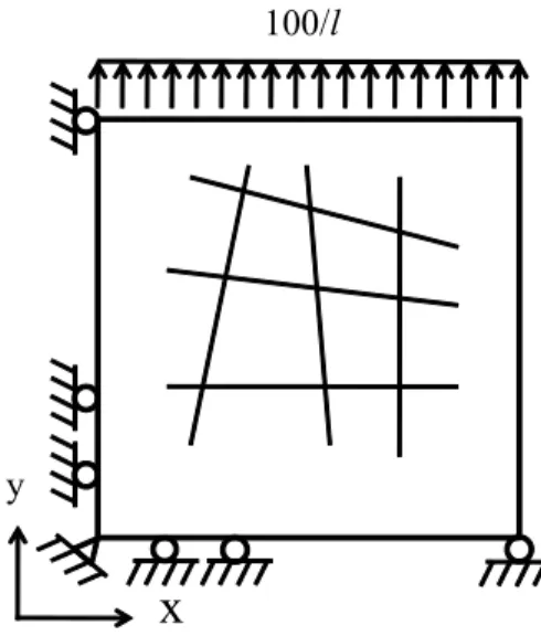
Fig. 1 An example square plate

[ ]

^T

Cov U =ε ⎡⎣Δ ΔU U ⎤⎦

( ) ( )

( )

1

2 4

T

ε R

− ⎡

=K ⎢⎣ −ϒ + ϒ + ϒ U U^μ ^μ

( ) ( )

(

^{−ϒ + ϒ + ϒ}^RV ² ⁴

)

^T^⎤_⎥⎦^K⁻^T

( ) ( )

{

1

2 2

T T T T

RV RV

ε ε

− ⎡ ⎤ ⎡ ⎤

=K ⎣ϒ U U^μ ^μϒ ⎦− ϒ⎣ U U^μ ^μϒ ⎦

( )⁴ ^T ^T( )⁴ ² ( )² ^T ( )^T⁴

}

^T

ε⎡ ⎤ ε⎡ ⎤ ⁻

− ϒ⎣ U U^μ ^μϒ ⎦− ⎣ϒ U U^μ ^μϒ ⎦ K ₍₂₉₎

As far as ϒRV is concerned, we can note that ,( )

e

r er

X K μ is equivalent to Δk)

in Eq. (22). Thus, the first term in Eq. (29) can be written as

T T

RV RV

ε ⎡⎣ϒ U U^μ ^μϒ ⎤⎦=ε ⎡⎣Δk U U k)_i ^μ ^T^μΔ)_j⎤⎦

(

⁴^k ¹ ( )ⁱ^k

)

^T

(

⁴^l ¹ ^{( )}^j^l

)

ε⎡ ₌ ₌ ⎤

= ⎢⎣

∑

Δ^k ^{U U}^μ ^μ

∑

Δ^k ⎥⎦

4 4

1 1

i jk l

Ω Ω = =

=

∫ ∫ ∑∑

( )

^{( )}

( )

^{( )} ^{( )}

{

^{ε ⎡}⎣^f ^k xⁱ ^f ^l x^j ^⎤⎦k U U k%ⁱ^k ^μ ^T^μ%^j^l

}

^d^{Ω Ω}^j^d ⁱ ₍₃₀₎

The detailed form of Δk) in Eq. (30) is given in Eqs.

(20) and (21). Based on the evaluation for respective finite elements, the remaining three other terms in Eq. (29) can be evaluated as follows:

( )i ^T ( )^Tj

ε ⎡⎣ϒ U U^μ ^μϒ ⎤⎦

( )

, ,

1 1

i j

e RV e RV

N N T

N N

e e

s es t et

e s e t

X X

= =

⎛ ⎞⎛ ⎞

⎜ ⎟⎜ ⎟

=⎜⎝

∑ ∑

^K _μ^U^μ⎟⎜⎠⎝

∑ ∑

^K _μ^U^μ⎟⎠

( )

^{( )}

1 e

e

N i e i

ff e e

e

R d

= Ω

⎛ ⎞

=⎜ Ω ⎟

⎝

∑∫

^{ξ k}^% ^U^μ⎠

( )

^{( )}

1 e

e N T

j e j

ff e e

e

R d

= Ω

⎞⎛ ⎞

⎟⎜ Ω ⎟

⎠⎝

∑∫

^{ξ k}^% ^U^μ⎠ ⁽³¹⁾ where k%^{e i}^{( )}=B E B^T ^{( )}ⁱ . With the aids of Eqs. (30) and (31), the evaluation of the covariance is completed.

4. Example analyses

As an example, we choose a square plate with dimension of 10×10m(Fig. 1). The material properties

assumed for the rectangular plate are E1=137.9Gpa and E2 =8.96GPa. The Poisson’s ratio is assumed as μ =0.30, and shear moduli in each corresponding direction are G23=6.21GPa, and G G31, 12_=7.1GPa,

respectively. The material properties correspond to the Graphite-Epoxy(AS3501). The thickness is h=0.1.

We employ two types of loadings: a distributed load of 10N in the direction normal to the plane of the plate(z-direction), and a distributed in-plane load in y-direction having value of 100N per unit length. The boundary condition is simple along left and bottom edges and free along right and top edges.

The stacking sequence for respective lamina is

(θ θ/− )4 for angle-ply laminate. The subscript 4 denotes the number of repetitions. The stacking schemes can be divided into two categories: symmetric stacking (θ θ/− ) (2 −θ θ/ )2 and asymmetric stacking

(θ θ θ θ/− ) (2 /− )2. As lamina angles, θ =30°, 45° are employed. If the stacking angles cross each other as (θ θ/− )4=(0 / 90− )4, it is called cross-ply laminates.

For the indirect consideration of the randomness in the random Poisson’s ratio, the auto-correlation function of the following type is used(See Eq. (35)).

These types of functions are generally accepted in the stochastic mechanics in representing randomness in the material properties having characteristics of exponential decaying correlation for the two distinct

(7)

Log of correlation distance d

COV (x-displacement)

-2 -1 0 1 2 3 4

0 0.02 0.04 0.06 0.08 0.1

0.12 Gr-Ep(AS/3501) (30/-60)a (30/-60)s (45/-45)a (45/-45)s (0/90)a (0/90)s

COV (x-displacement)

-2 -1 0 1 2 3 4

0 0.02 0.04 0.06 0.08 0.1

0.12 Gr-Ep(AS/3501) (30/-60)a (30/-60)s (45/-45)a (45/-45)s (0/90)a (0/90)s

(a-1) COV of displacement in x direction: proposed scheme

(a-2) COV of displacement in x direction: MCS

COV (y-displacement)

-2 -1 0 1 2 3 4

0 0.0002 0.0004 0.0006 0.0008 0.001 0.0012

Gr-Ep(AS/3501) (30/-60)a (30/-60)s (45/-45)a (45/-45)s (0/90)a (0/90)s

COV (y-displacement)

-2 -1 0 1 2 3 4

0 0.0002 0.0004 0.0006 0.0008 0.001 0.0012

Gr-Ep(AS/3501) (30/-60)a (30/-60)s (45/-45)a (45/-45)s (0/90)a (0/90)s

(b-1) COV of displacement in y direction(in-plane loading direction): proposed scheme

(b-2) COV of displacement in y direction(in-plane loading direction): MCS

COV (z-displacement)

-2 -1 0 1 2 3 4

0 0.0015 0.003 0.0045 0.006 0.0075 0.009

Gr-Ep(AS/3501) (30/-60)a (30/-60)s (45/-45)a (45/-45)s (0/90)a (0/90)s

COV (z-displacement)

-2 -1 0 1 2 3 4

0 0.0015 0.003 0.0045 0.006 0.0075 0.009

Gr-Ep(AS/3501) (30/-60)a (30/-60)s (45/-45)a (45/-45)s (0/90)a (0/90)s

(c-1) COV of displacement in z direction(out-of plane direction): proposed scheme

(c-2) COV of displacement in z direction(out-of plane direction) : MCS

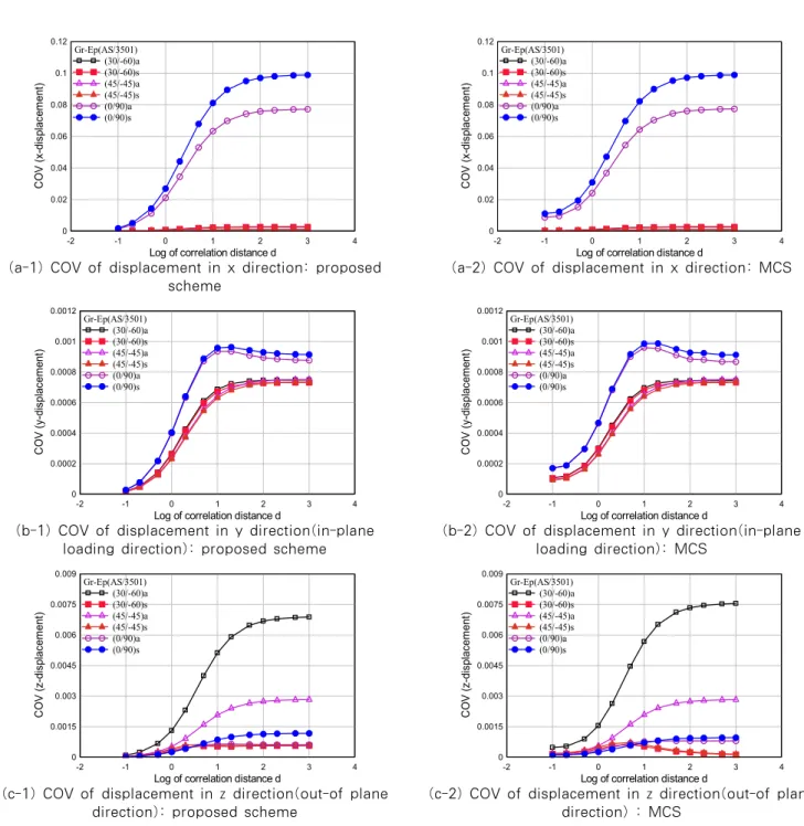
Fig. 2 Response variability of example plate points in the domain.

( )

²ff ^{⁽ ^x ^y⁾^/^d^}

R ξ =σ e⁻^ξ ⁺^ξ ⁽³²⁾

The function given in Eq. (35) is used not only in the proposed formulation bus also in the MCS.

Actually, the MCS is used to verify the performance of the proposed scheme. The variance of the stochastic field is denoted as σ²ff, and the correlation distance which specifies the fluctuation feature of the stochastic

field is represented with symbol d. The vector

(

^{ξ ξ}^x^, ^y

)

is the relative distance vector between two points in the domain. We choose σff=0.1 throughout the analysis.

4.1 Comparison with MCS

The coefficient of variation(COV) of responses is evaluated at the upper-right corner of the plate(See Fig. 1). In order to avoid the complexity of presentation, the results from the proposed scheme and those from

(8)

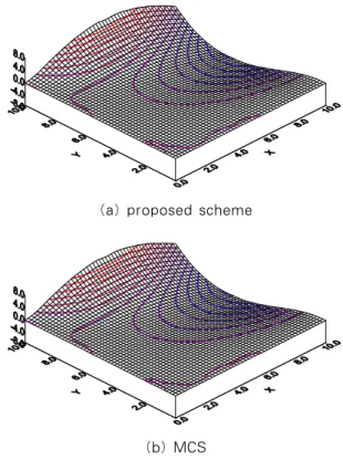
(a) proposed scheme

(b) MCS

Fig. 3 Plots of mean displacements in z-direction the MCS are given separately.

In Fig. 2, the subscripts ‘s’ and ‘a’ signify symmetric and asymmetric stacking scheme, respectively, and the values in the parentheses are stacking angles.

Globally, a good agreement between the proposed scheme and the MCS is observed with the trend of having slightly larger values in MCS than the proposed scheme.

As noted in Fig. 2, the COV for the cases of cross-ply laminates((0/90)a and (0/90)s) in the x-displacement show larger values than the other cases. In fact, this result is expected in advance because we consider only the randomness in the Poisson’s ratio. That is, the response variability is to be larger for the in-plane response especially in the direction normal to the loading (i,e, in the x-direction) than in the loading direction. The maximum value of COV is observed to be the same as the COV of the stochastic field, 0.1.

In some cases such as y-displacement for cross-ply and z-displacement for symmetric stacking scheme, the COV shows a trend of decrease as the correlation distance increases. From these results we can note that the response variability of composites is not a monotonic function of the correlation distance ^ of the stochastic field. Though the maximum value of COV is equal to the COV of the stochastic field, it is revealed that the COV is smaller for the composite plates than that of the isotropic plate(Noh, 2004), where about 20% of the COV of stochastic field has been observed.

4.2 Distribution of standard deviation and COV

In order to have insight on the response variability of composite laminates, we compare the standard deviation(SD) and COV of the displacement components over the entire domain. The respective values of SD and COV are shown as ordinate of the corresponding point in the domain. Here, the material has the following properties: E1=38.61Gpa, E2= 8.274GPa, μ =_0.26, G₂₃=3.45GPa, and G G31, 12

=4.14GPa. The stacking scheme is (20/110)²(20/110)²,

thus it is cross-ply asymmetric case. The correlation distance for the analysis is d=20.0.

According to Eq. (19), the mean stiffness of the structure is different from the deterministic one due to the effect of even power of stochastic field function.

Therefore, the mean displacement in Fig. 3 differs from the deterministic one. However, the result of the proposed scheme is almost the same as the MCS, as shown in Fig. 3.

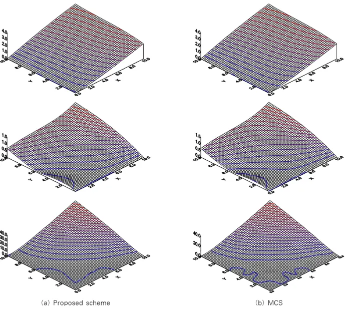
In Fig. 4, the fields of SD of the displacement components are shown. With a minor difference, two analysis results are in good agreement.

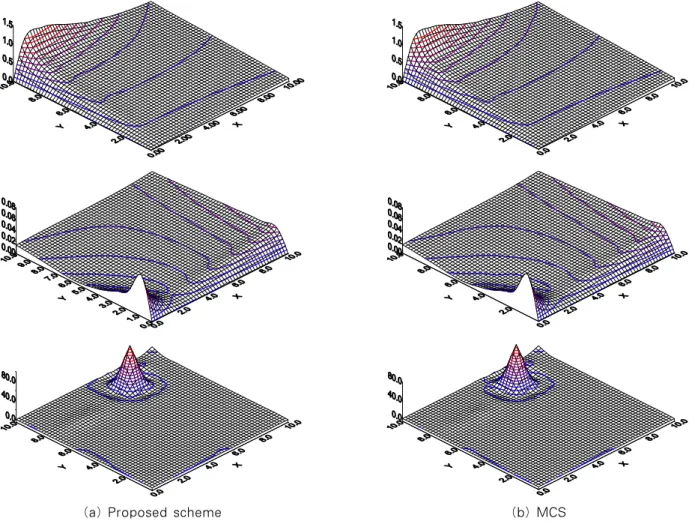
The COV fields of displacement of each displacement components are shown in Fig. 5 for the proposed scheme and MCS. As seen in the figures, the overall trend coincides with each other within a minor difference. In case of the displacement in z-direction, we can observe a peak in COV at a specific location.

The reason for this can be found when we look into Figs. 3 and 4 closely; even though the SD field takes normal pattern of variation in the domain, the mean displacement has some fluctuation, which is caused by the torsion effect due to material asymmetry. Since

(9)

(a) Proposed scheme (b) MCS

Fig. 4 Plots of standard deviation of the displacement in x, y, z directions

the COV is the ratio of SD to the mean, the COV can have a peak if the mean tends to zero. Therefore, the COV variation of z-displacement has a peak which is relatively high when compared with the other points in the domain. However, even in this case, a good agreement between two analyses is observed.

4.3 Effect of change in stacking angle

For the investigation of the effect of the stacking scheme, we take the stacking angle as a variable. The stacking scheme of laminae for the example composite plates is (θ/θ+90)4 in an asymmetric manner, and the value of θ in degree changes from 0 to 90. The material properties are the same as used in the section 4.2.

The COV is found at the upper-right corner of the plate.

As seen in Fig. 6, the COV varies as the lamination angle changes. Depending on the displacement compo- nent, COV is affected in different manners. The minimum value of COV is found at the lamination angle of 50 in the case of x-displacement. In the case of z-displacement, however, there appears a peak around angle of 20 degree. In fact, this COV corresponds to the value at the upper-right corner of Fig. 5

4.4 Computational efficiency

The computational efficiency of the proposed scheme can be estimated from the investigation of the CPU

(10)

(a) Proposed scheme (b) MCS Fig. 5 Plots of COV in x, y, z displacement

Stacking angle (degree)

COV of response

0 15 30 45 60 75 90

0 0.02 0.04 0.06 0.08 0.1 0.12

Correlation distanace d = 20.0 COVx - Proposed COVy - Proposed COVx - MCS COVy - MCS

Stacking angle (degree)

COV of response

0 15 30 45 60 75 90

0 0.2 0.4 0.6 0.8 1 1.2

Correlation distanace d = 20.0 COVz - Proposed COVz - MCS

Fig. 6 Effects of stacking schemes

time for one batch analysis. For the proposed scheme, around 105 seconds are needed to obtain the COV of response. This, in fact, corresponds to the 276 times of deterministic analysis, which means that the proposed scheme is equivalent to the MCS analysis with 276 samples. However, in the MCS it is not unusual to use thousands of and even more samples to match the pre-assigned statistical terms. Based on these observations, we can attest that the proposed scheme has greater efficiency than the conventional Monte Carlo analysis.

5. Conclusions

In order to investigate the effect of random Poisson’s ratio in the laminate composite plates, we proposed a stochastic finite element analysis formulation.

The constitutive coefficients including the Poisson’s ratio in its fraction form are transformed into the

(11)

power-series in terms of the stochastic field function in ascending order, which enable us to establish formulae to obtain response statistics.

Contrary to the common sense that the composite might have higher degree of uncertainty in response, it is observed that the response variability is relatively small than the case of plate in isotropic material. In general, the COV of the response is obtained to be less than 10% of the COV of stochastic field. However, due to the skew effect of asymmetrical material, the out of plane behavior has some irregularity causing a peak in COV. The maximum COV, if we do not take into account the peak, appears in the direction normal to the loading revealing equal value of COV of stochastic field when correlation distance is very large, especially in the symmetrically stacked cross-ply laminates.

It is shown that the proposed scheme is more efficient than the conventional MCS analysis in terms of CPU time. Moreover, the proposed scheme yields a good agreement with Monte Carlo analysis. It shows the adequacy of the proposed scheme in the estimation of response variability of laminated composite plates.

Based on the fact that the elastic modulus is the parameter that governs the behavior of structures, it is needed to take into account the random elastic modulus in evaluating the response variability.

References

Choi, C.K., Noh, H.C. (2000) Weighted Integral SFEM Including Higher Order Terms, Journal of Engineering Mechanics, ASCE 126(8), pp.859~866.

Deodatis, G., Shinozuka, M. (1989) Bounds on Response Variability of Stochastic Systems, Journal of Engineering Mechanics, 115(11), pp.2543~2563.

Hilton, H.H., Yi, S. (1999) Stochastic Delamination Simulations of Nonlinear Viscoelastic Composites During Cure, Journal of Sandwich Structures and Materials, 1, pp.111~127.

Noh, H.C. (2004) A Formulation for Stochastic Finite Element Analysis of Plate Structures with Uncertain

Poisson’s ratio, Comput. Methods Appl. Mech.

Engrg. 193(45~47), pp.2687~2718.

Kam T.Y., Lin S.C., Hsiao K.M. (1993) Reliability Analysis of Nonlinear Laminated Composite Plate Structures, Composite Structures, 25, pp.503~510.

Leddy, J.N. (1997) Mechanics of Laminated Composite Plates, theory and analysis, CRC Press, Inc.

Lekou, D.J., Philippidis T.P. (2008) Mechanical Property Variability in FRP Laminates and its Effect on Failure Prediction, Composites: Part B, 39, pp.1247~1256.

Chen, N.Z., Guedes S.C. (2008) Spectral Stochastic Finite Element Analysis for Laminated Composite Plates, Comput. Methods Appl. Mech. Engrg. 197, pp.4830~4839.

Onkar, A.K., Upadhyay, C.S., Yadav, D. (2007) Probabilistic Failure of Laminated Composite Plates using the Stochastic Finite Element Method, Composite Structures, 77, pp.79~91.

Onkar, A.K., Yadav, D. (2004) Non-linear free Vibration of Laminated Composite Plate with Random Material Properties, Journal of Sound and Vibration, 272, pp.627~641.

Singh, B.N., Bisht, A.K.S., Pandit, M.K., Shukla, K.K. (2009) Nonlinear free Vibration Analysis of Composite Plates with Material Uncertainties: A Monte Carlo Simulation Approach, Journal of Sound and Vibration, 324, pp.126~138.

Stefanou, G., Papadrakakis, M. (2004) Stochastic Finite Element Analysis of Shells with Combined Random Material and Geometric Properties, Computer Methods in Applied Mechanics and Engineering, 193(1~2), pp.139~160.

Wang, F.Y. (1990) Monte Carlo Analysis of Nonlinear Vibration of Rectangular Plates with Random Geometric Imperfections, International Journal of Solids and Structures, 26(1), pp.99~109.

논문접수일 2010년 11월 9일

논문심사일 2010년 11월 12일

게재확정일 2010년 11월 29일