IEG 환경지질연구정보센터

(1)

Vol. 12, No. 3, p. 255−264, September 2008 DOI 10.1007/s12303-008-0026-5

Estimating apparent thermal diffusivity using temperature time series: A com- parison of temperature data measured in KMA boreholes and NGMN wells

ABSTRACT: Two different time series data sets, shallow ground temperatures of 58 synoptic stations of the Korea Meteorological Administration (KMA) and groundwater temperatures of 67 wells of the National Groundwater Monitoring Network (NGMN), were analyzed to estimate the apparent thermal diffusivity by using the analytical solution of the one-dimensional heat conduction equation. The KMA temperature data measured at 1-5 m depths illustrated values of the phase delay and the amplitude decay coincident with their theoretical relationship, indicating that the conductive heat transport should prevail over the nonconductive processes.

On the contrary, some of the estimates from temperatures at a depth of 0.5 m were away from the theoretical values. It is most likely that the deviation would be caused by the effects of latent heat associated with freezing and thawing of the near ground surface. In contrast to KMA data, results obtained from the NGMN data highly deviated from the theoretical ones, and thereafter yielded unacceptably high values of thermal diffusivities as compared to the representative values of soils and rocks. Implication of the discrepancy between two data sets was discussed in con- junction with perturbation of the conductive heat transport by free convection of water and air occurring in large diameter wells as well as the convective heat transport by groundwater flow.

Key words: apparent thermal diffusivity, temperature time series, heat conduction model, critical geothermal gradient, KMA, NGMN 1. INTRODUCTION

Temperature measurements in boreholes are quite simple and can be easily performed to get vertical profiles or time series data. Furthermore, equipments for measuring temperature in boreholes are readily available within the accuracy of ± 0.01°C. There have been many attempts to use the subsurface temperature with a variety of applications in hydro- geology. It has been used as a tracer for analyzing the concurrent flow of heat and water along vertical profiles of the subsurface medium to elucidate vertical groundwater movement (Bredehoeft and Papdopulos, 1965), groundwater recharge (Taniguchi and Sharma, 1993; Tabbagh et al., 1999), percolation rates in the vadose zone (Constantz et al., 2003) and the pattern of groundwater discharge in a streambed (Conant, 2004). Anderson (2005) presented a

comprehensive review on the application of temperature to a variety of hydrogeological settings. Recently, ground temperature data have been vigorously used in reconstructing past climate changes (Lachenbruch and Marshall, 1986;

Veliciu and Safanda, 1998; Huang et al., 2000; Cermak and Bodri, 2001; Dorofeeva et al., 2002; Gosselin and Mare- schal, 2003).

Temperature measurements in shallow vadose environments are mainly used in agronomical studies to character- ize soil properties (Passerat de Silans et al., 1996; Verhoef et al., 1996) and the thermal regime of the active layer above permafrost (Hinkel, 1997; Hinkel et al., 2001). Tem- perature time series data measured in soils at a shallow depth generally show annual cyclic variations, which can be effectively described by the one-dimensional heat conduction model. The thermal diffusivity is the key parameter that controls the temperature in soils near the ground surface where periodic temperature change is progressively attenuated and delayed with depth. The investigation of soil temperature variations has practical applications in agricultural engineering, since it can lead to the evaluation of opti- mum conditions for plant growth and development, and also can be used for the control of the thermal-moisture regime of soil (Usowicz et al., 1996). It is also an important parameter in designing the geothermal heat pump system, in which extraction of thermal energy is accomplished by using a ground heat exchanger (GHE). The heat transfer between the GHE and the surrounding geological forma- tions occurs primarily by conduction. Thus, the effective thermal diffusivity of the ground is the fundamental parameter in determining a required length of the GHE (Kavanaugh and Rafferty, 1997). Lee (2006) analyzed characteristics of ground and groundwater temperature data measured in Seoul, a metropolitan city of Korea, as a basic feasibility study for geothermal heat pumps.

The thermal diffusivity of soils and rocks can be obtained from laboratory experiments (Moench and Evans, 1970;

Stephenson, 1987, Bristow et al., 1994; Kluitenberg et al., 1995) which, however, often yield unsatisfactory results since they usually deal with a small size sample in spite of Min-Ho Koo*

Yoonho Song Department of Geoenvironmental Sciences, Kongju National University, Chungnam 314-701, Korea Groundwater and Geothermal Resources Division, Korea Institute of Geoscience and Mineral Resources (KIGAM), Daejeon 305-350, Korea

*Corresponding author: [email protected]

(2)

heterogeneities of the real field. Furthermore, in the case of soils, it is difficult to take undisturbed samples as preserved as the natural condition of the materials. Therefore, field- measured ground temperature data have been widely used as an alternative to estimatethe thermal diffusivity (Adams et al., 1976; Asrar and Kanemasu, 1983). Horton et al. (1983) analyzed the limitations of the different methods to calculate the thermal diffusivity in terms of the calculated results and forthe quantity and quality of data required to make the calculations.

Most approaches in the literature to use subsurface temperatures assume that temperatures measured in a borehole should be in equilibrium with the surrounding media. How- ever, it has long been recognized that the fluids within open boreholes, air and water, are subject to being unstable by free convection, provided that the thermal gradient exceeds a certain critical value (Krige, 1939). Convection within the borehole causes borehole temperatures to be different from the surrounding media, and thereafter misleads the inter- pretation of temperature data. Diment (1967) and Gretener (1967) presented observational evidence that water in large diameter wells was unstable under the normal geothermal gradient as predicted by the Krige’s formulation. Thus, it might be inappropriate to use temperature data measured in large diameter wells to interpret the hydrothermal process occurring in the subsurface, since the condition of thermal equilibrium between the borehole and the surrounding medium could be invalidated by convection.

The primary objective of this paper is to analyze the apparent thermal diffusivity from two different time series data sets: shallow ground temperatures of the Korea Mete- orological Administration (KMA) measured in small diameter boreholes and groundwater temperatures of the National Groundwater Monitoring Network (NGMN) measured in large diameter wells. Estimation of the thermal diffusivity in the literature has been performed mostly by using soil temperature data in the unsaturated zone, but seldom by groundwater temperature data. Thus, the motivation of this study is to compare the results of two different data sets and further discuss their implications in association with free convection of fluids within boreholes as well as the convective heat transport due to groundwater flow.

2. METHODS AND MATERIALS 2.1. Theoretical background

The governing equation describing one-dimensional conductive heat transfer in a homogeneous medium is

(1) where T is temperature, t is time, z is the depth from the ground surface taken as positive downward and α is the thermal diffusivity of the bulk medium. When the equation

is concerned with the underground medium where both conductive and nonconductive heat transfer processes occur, α is usually called the ‘apparent’ or ‘effective’ thermal diffusivity. The nonconductive heat transfer includes convection driven by water and vapor transport, phase changes and associated latent heat. Although heat transfer in the subsurface is dominated by conduction, it is recognized that the nonconductive processes also play a comparably important role particularly in the near ground surface. Thus, the estimated apparent thermal diffusivity can be very different from the real value associated with conduction.

Furthermore, if the vadose zone is concerned, the conductive process becomes quiet complicated in itself, being affected by presence of water. The vadose zone undergoes temporal variation of the thermal diffusivity due to associated variation of its water content driven by precipitation and evapotranspiration. Soils with higher water contents tend to have higher thermal diffusivities. Therefore, the heat conduction model based on the assumption of time-invariant diffusivity can only give approximate results of temperature variation. Conversely, the estimated thermal diffusivity based on the model of time-invariant diffusivity should be interpreted as an average value over the period of measurements. Thus, the unsaturated flow leads to a complicated process of heat transfer in the vadose zone by causing spa- tiotemporal variation of thermal properties as well as convective heat transfer.

Based on temperature time series data, the apparent thermal diffusivity can be determined by analytical or numerical solutions of Equation (1) with the assumption of constant diffusivity. Horton et al. (1983) investigated several methods available for determining the apparent thermal diffusivity of soil near the ground surface from soil temperatures.

Zhang and Osterkamp (1995) discussed some considerations of finite difference methods in determining the thermal diffusivity from a temperature time series. Analytical methods are used in this study to estimate the apparent thermal diffusivity.

In order to get the analytical solution of Equation (1), the periodic oscillations of the ground surface temperature, expressed as a Fourier series, can be used for a boundary condition;

(2) where T₀ is the average ground surface temperature, ω is the fundamental angular frequency, A_n is the amplitude and φn is the phase. The analytical solution of Equation (1) with a time-periodic surface temperature of Equation (2) in a semi- infinite half-space is;

(3) It appears from Equation (3) that there are some analyt-

∂ T

---∂ t α∂²T

∂ z² ---

=

T_s( ) Tt 0 A_nsin n( ωt φ+ n)

n 1=

∑M

+

=

T z t( ) T, 0 A_ne^–^{z nω 2α}^⁄ sin n( ωt φ+ n–z nω 2α⁄ )

n 1=

∑M

+

=

(3)

ical expressions available to determine the apparent thermal diffusivity: the phase equation, the amplitude equation and the logarithmic equation.

Under the assumption of a periodic surface temperature with the fundamental angular frequency (M=1), the phase equation to determine apparent thermal diffusivity can be derived explicitly from the argument of the trigonometric term in Equation (3);

(4) where δt is the phase difference between temperature variations at the two depths z₁ and z₂. Three methods are available to calculate the phase difference from two temperature time series measured at different depths. First, the phase delay can be calculated from the sinusoidal functions best- fitted to the measured temperatures by applying the least square method. Secondly, it can be obtained from the time interval between measured occurrences of the maximum temperature (Horton et al., 1983). Lastly, a cross-correlation analysis, which is used in this study, can also yield the phase difference of two temperature time series (Koo et al., 2003).

Under the assumption made above for the phase equation, the amplitude equation to determine apparent thermal diffusivity can be derived explicitly from the argument of the exponential term in Equation (3);

(5) where ΔT1 is the amplitude at z₁ and ΔT2 is the amplitude at z2. Similar methods are also available to calculate the amplitudes. First, the sinusoidal functions best-fitted to the measured temperatures can be also used to get the amplitudes.

Secondly, they can be approximated from the minimum and maximum temperature readings over a period of the fundamental cycle (Hinkel, 1997). Lastly, the amplitude ratio can be directly obtained from a linear regression analysis of two temperature time series in which the phase difference, determined by the cross-correlation analysis, is taken into account

to nullify the phase delay (Koo et al., 2003). The last method is used in this study.

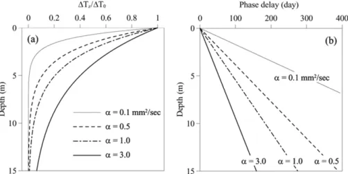
Figure 1 is the calculated results from Equations (4) and (5) illustrating how the amplitudes of the temperature variations decay and how the phases are delayed with depth depending on the thermal diffusivity. Representative values of the thermal diffusivity for various soils and rocks range between 0.2 and 1 mm²/sec (Carslaw and Jaeger, 1959).

Thus, it is highly likely that the ground temperatures up to a depth of 10 m would exhibit discernible annual fluctua- tions, and could be utilized to determine the apparent thermal diffusivity.

Combining Equations (4) and (5) yields the relationship between the phase delay and the amplitude ratio;

(6) The phase delay and the amplitude ratio estimated from two temperature time series at different depths should fol- low the theoretical relationship as given in Equation (6), provided that the temperature field is not highly disturbed by the nonconductive processes of heat transfer. Using both synthetic and measured time series of temperature data, Koo et al. (2003) analyzed effects of the vertical water flow in the vadose zone on the estimates of thermal diffusivity.

In their numerical results, effects of the water flow were evidently reflected in the amplitude decay to increase the apparent thermal diffusivity. On the contrary, the estimates obtained from the phase equation gave a remarkably accu- rate result regardless of occurrence of the water flow.

2.2. Materials

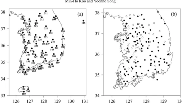
The apparent thermal diffusivities of the shallow ground in Korea are analyzed by using ground temperature data measured at 58 synoptic stations of KMA and groundwater temperature data measured at 264 wells of NGMN consist- ing of 169 bedrock wells and 95 alluvial wells (Fig. 2).

The ground temperature, a surface observatory element of

α 1

2ω --- z₂–z₁

δt ---

2

=

α ω----2 z₂–z₁ ΔT1⁄ΔT2

( )

ln---

2

=

ΔT2⁄ΔT1

( )

ln = –ω tδ

Fig. 1. Annual variations of the subsurface temperature calculated from the solution of one-dimensional heat conduction equation: (a) the amplitude decay and (b) phase delay with depth.

(4)

meteorological parameters, is being measured at the synoptic stations of KMA. It is measured at several depths in steel boreholes with an inner diameter of 4.2 cm. The analysis was made for the temperature data over the period from 1981 to 2002 measured at depths of 0, 0.5, 1, 1.5, 3 and 5 m on a daily basis. All of the data were preprocessed to pro- duce temperature time series with a sampling interval of 24 hours. A prior process of quality control for raw data was conducted to eliminate some unacceptable values which were thought to be associated with wrong readings or inputs by mistake. The elimination was performed by a simple numerical scheme where the temperature under inspection is regarded as a bad data, if it is higher or lower than the temperature of the previous day by more than 15 °C.

Under the ‘Master plan for groundwater management’ of the Ministry of Construction and Transportation (MOCT) in 1996, the Korea Water Resources Corporation (KOWACO) has constructed NGMN to measure and compile nationwide data on water level, temperature and electrical conductivity of groundwater. NGMN operates an automated measuring system on a 6-hour basis. All the data are being collected, analyzed and provided by the National Groundwater Infor- mation Management and Service Center (GIMS) in KOWACO which was established in 2003. Temperature data of 264 monitoring wells which had been installed from 1995 to 2000 were obtained from GIMS, and the data measured from the beginning of measurements to December of 2001 were used for the analysis.

3. RESULTS AND DISCUSSION 3.1. Analysis of KMA temperature data

In order to estimate the apparent thermal diffusivity of

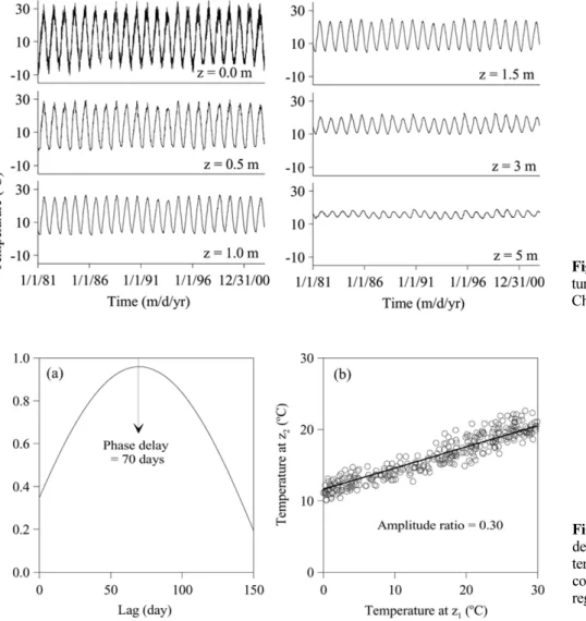
soils at various depths of KMA stations, the phase and amplitude equations are applied to time series data of ground temperatures. Figure 3 shows temporal variation of ground temperatures at various depths measured at the Chuncheon station. A clear illustration of the amplitude decay and the phase delay is observed in the figure, indicating that conduction is the dominant mechanism of heat transfer in the shallow ground. As discussed above, the phase delay between two temperature time series is determined by a cross-correlation analysis (Fig. 4a), and the apparent thermal diffusivity is calculated by Equation (4).

The amplitude decay is also determined by a linear regression analysis of two time series of which the phase delay is nullified (Fig. 4b), and the apparent thermal diffusivity is calculated by Equation (5).

Figure 5 shows estimates of the phase delay and the amplitude decay between temperatures at the ground surface (z₁) and temperatures at the depths of 0.5, 1, 1.5, 3 and 5 m (z₂) determined for 58 KMA stations. The solid line in Figure 5 represents the theoretical relationship between the phase delay and the amplitude decay as given in Equation (6) derived from the solution of one-dimensional heat conduction equation. Most of the estimates for temperatures at depths equal to or greater than 1 m fall closely on the theoretical curve, indicating that the conductive process of heat transfer prevails over the nonconductive processes in the associated depth intervals. Therefore, the estimated apparent diffusivity should be quite close to the intrinsic diffusivity.

On the contrary, some of the estimates for temperatures near the ground surface (0.5 m) are far away from the theoretical curve. The most likely possibility is that the nonconductive heat transfer would occur actively near the ground surface, and thereby could cause a temperature vari- Fig. 2. Location maps of (a) surface synoptic stations of KMA and (b) monitoring stations of NGMN: closed circles represent the monitoring stations with both alluvial and bedrock wells, and open circles represent the stations with a bedrock well only.

(5)

ation to deviate from the theoretical one based on the heat conduction model. As would be expected, soils near the ground surface are highly vulnerable to freezing and thawing, convective heat transfer due to infiltrated water and temporal variation of thermal properties. As illustrated in Figure 5, the deviation associated with the nonconductive heat transfer seems to lead to a reduction of the phase delay.

Although not directly explored in this paper, the link between the nonconductive heat transfer and reduction of the phase delay could be examined by a numerical model of heat transfer incorporating convection, phase changes and associated latent heat.

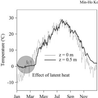
Figure 6 shows a clear evidence of the nonconductive heat transfer, illustrating variation of the ground temperature affected by latent heat associated with freezing and thawing. During the months of the year when freezing and thawing of the ground surface occur (January – March), the ground temperature at a depth of 0.5 m is immune to change being affected by the latent heat released or absorbed during phase changes. Thus, the effect of latent heat in the cold season highly disturbs the conductive temperature variation observed in the other seasons. The per-

Fig. 3. Variations of ground temperature measured at various depths of the Chuncheon station.

Fig. 4. Determination of the phase delay and the amplitude ratio of two temperature time series by: (a) a cross correlation analysis and (b) a linear regression of the two data sets.

Fig. 5. Estimated phase delay and amplitude damping with depth:

the solid line represents theoretical values calculated from the solution of one-dimensional heat conduction equation.

(6)

sistence of a constant temperature close to zero degree is directly related to soil water content. It is intuitive that soils with higher water contents would undergo the latent heat effect for longer period of time. Soils with smaller particles generally have higher water contents due to their higher field capacity and lower permeability. Thus, it is probable that the latent heat effect would be more pronounced in fine-grained soils. In addition to the latent heat effect, freezing and thawing of soils also can affect the process of conductive heat transfer by contrasting thermal diffusivities of water (0.14 mm²/sec) and ice (1.2 mm²/sec). Thus, the heat transfer in soils near the ground surface is a very complicated process, being affected by the presence of water and its phase changes in the cold season. As mentioned earlier, the heat conduction model based on the assumptions of constant diffusivity and no heat source/sink only gives approximate results, which sometimes lead to erroneous predictions depending on the degree of discrepancies between the assumed and the real field situations.

Conclusively, it appears from Figure 5 that availability of

the phase and amplitude equations based on the simplified heat conduction model to determine the apparent thermal diffusivity may be limited particularly for soils near the ground surface in Korea. In consideration of the results discussed above, it is likely that the limited availability would be associated with the freezing and thawing process as well as the convective heat transfer of water and air which is not directly accounted for in this paper. These nonconductive processes generally are more prominent in the top soils within 0.5 m depth below the ground surface.

Figure 7 shows variations of the apparent thermal diffusivity of KMA soils with depth determined by the amplitude equation. Figure 7a represents thermal diffusivities for the depth intervals illustrated by arrow lines, and Figure 7b represents thermal diffusivities for the whole intervals from the ground surface to the depths given in y-axis. The results clearly demonstrate that soils at greater depths would have higher thermal diffusivities. Particularly the drastic increase can be observed at a depth of 1 m. As discussed in Koo et al. (2003), variability of the apparent thermal diffusivity should be attributed to the distinctive differences in the porosity, the water content and the organic content of soils.

Thus, it is likely that low diffusivities observed in the top soils would be caused by high porosities due to less com- paction and development of the aggregate structure, low water contents driven by evaporation and high organic contents as compared to the underlying soils. The estimated diffusivity is regarded as an outlier if it is higher than the upper quartile by more than 1.5 times of the interquartile range (IQR). It is not clear whether the outliers shown at shallow depths represent actual diffusivities or not. How- ever, the outliers plotted in Figure 7a are much higher than the representative values of soils in the literature (Carslaw and Jaeger, 1959).

3.2. Analysis of groundwater temperature data of NGMN 3.2.1. Analyzing quality of data

Monitoring data of groundwater temperature in 169 bedrock wells and 95 alluvial wells of NGMN are used to estimate the apparent thermal diffusivity. The average installation Fig. 6. Variations of surface and ground temperatures showing the

effect of latent heat associated with freezing and thawing of the near ground surface (Chuncheon KMA station).

Fig. 7. Variations of the estimated thermal diffusivity with depth: each box- whisker plot represents thermal diffusivities for (a) the depth interval illustrated by arrow lines and (b) the interval from the ground surface to the depth given in y-axis.

(7)

depths of bedrock and alluvial wells are 70 m and 20 m, respectively. Data loggers of the alluvial wells are mostly placed at depths from 5 m to 10 m below the ground surface, depending on the well depth and the water level. Most data loggers of the bedrock wells are placed at a depth of 20 m. In consideration of the depths of temperature measurements, it is expected from Figure 1 that a periodic temperature variation with discernible amplitude would be observed in the alluvial wells; meanwhile it may or may not be noticeable in the bedrock wells. Thus, if the conductive heat transfer prevails in the subsurface of monitoring wells, groundwater temperatures would be periodic or practically constant depending on the depth of measurements.

However, the expectation of steady periodicity or constancy has failed in many temperature data sets of NGMN.

The failure is thought to be mainly caused by malfunction of the data logger for a certain period of time. In spite of regular inspection of monitoring stations and prompt replacement of malfunctioning devices in the data logger, abnormal values or outliers often occur due to intrinsic limitations of automatic monitoring and transmission (Yi et al., 2005). Yi et al. (2005) analyzed NGMN data sets of monitoring wells in the Han River basin and found that the most prominent patterns of the outliers were rapid decline in water level, no variation in temperature and steep decline in electrical conductivity. However, inspection of the table summarizing the outliers in Yi et al. (2005) reveals that no variation in temperature is mostly found in the bedrock wells. As mentioned above, it is expected that the bedrock wells would show a periodic temperature variation with small amplitudes or a constant temperature due to a great depth of measurements. Thus, consideration of no variation as one of criteria to recognize outliers in temperature may lead to a wrong judgment, unless the depth of measurements is taken into account in the analysis.

In this study, temperature variations observed in 264 monitoring wells of NGMN are classified into three patterns. First, based on the speculation discussed above, temperature data sets showing periodicity or constancy for the whole period of measurements are considered normal or natural (Fig. 8a). Secondly, date sets showing irregular or abrupt changes and steady increase or decrease are considered abnormal or artificial (Fig. 8b). It is likely that abnormal variations occurred mainly due to malfunction of the data logger and partially due to artificial impacts such as groundwater contamination and nearby construction accom- panying ground excavation. Finally, date sets having abnormal variations for a certain period of time are considered mixed (Fig. 8c). The spikes in temperature observed in Fig- ure 8a and 8c are related to short-term disturbances by regular inspection of the data logger and pumping for well- maintenance and water sampling. The analysis for temperature data sets observed in 264 monitoring wells illustrates that the normal, abnormal and mixed variations are found in

171 (64.8%), 27 (10.2%), and 66 stations (25%), respectively.

The stations with normal variations comprise 85 stations with periodic variation and 86 stations with no variation.

The stations with mixed variations also show periodic variation (10 stations) as well as no variation (56 stations), if the fractions with abnormal variations are ignored.

3.2.2. Determination of the apparent thermal diffusivity Temperature data of the 95 monitoring stations showing periodic variations are used to estimate the apparent thermal diffusivity. For 10 data sets which contain abnormal variations in a partial period of time, the only fractions of data showing steady periodicity are used for the analysis. Deter- mination of the apparent thermal diffusivity requires another data set measured at a different depth, which is not available in the monitoring stations of NGMN. Thus, in spite of a crude analogy, the ground surface temperature measured at the nearest KMA station was inevitably used as an alternative. As would be expected, the discrepancy should lead to results with varying degrees of errors depending on the distance between the monitoring well and the nearest KMA station. The apparent thermal diffusivity is determined by the same procedure as the analysis of KMA data. In spite of the prior elimination of data with abnormal temperature measurements, the estimated results need a further refine- ment since they are flawed by the use of KMA data as an alternative to the surface ground temperature and some of data sets still contain less reliable measurements. Thus, in order to enhance quality of the analysis, some of data sets are additionally discarded if the correlation coefficient is Fig. 8. Patterns of temperature variation observed in the monitoring wells of NGMN: (a) normal (periodic or constant), (b) abnormal, and (c) mixed.

(8)

less than 0.8 in the linear regression analysis of two temperature time series to obtain the amplitude ratio. Finally, 67 data sets, which comprise 53 alluvial wells and 14 bedrock wells, are selected and used for estimating the apparent thermal diffusivity.

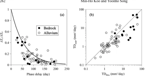
Estimates of the phase delay and the amplitude decay determined for 67 data sets are shown in Figure 9a where the solid line represents the theoretical relationship. In contrast to the results of KMA temperature data as given in Figure 5, many of the estimates highly deviate from the theoretical curve, falling mostly on the zone below the theoretical curve due to underestimation of the phase delay or the amplitude decay. The discrepancy indicates that the nonconductive heat transfer prevails over conduction in groundwater of the wells. Figure 9b shows the apparent thermal diffusivities estimated by the phase and amplitude equations. In the case of alluvial wells (open circles), some of the estimates are within the range of the representative values for soils and rocks, while others are not. On the contrary, all of the estimates for bedrock wells ranging between 2.2 and 58 mm²/sec are much higher than the representative values.

Consequently, the results suggested that the use of a periodic temperature time series to determine the thermal diffusivity should be highly limited when applied to the NGMN data, while it produced fairly reliable estimates for the KMA data. The inconsistency may be attributed to two distinctive features of the KMA and the NGMN data. First, the KMA data was measured at shallow depths in the vadose zone, while the NGMN data was measured at depths below the water table in the saturated zone. It is well known that the influence of groundwater flow plays a sig- nificant role on the temperature distribution of the subsurface. It also can disturb the patterns of periodic variations observed in the shallow underground. Thus, the NGMN data should be influenced by the convective heat transfer due to groundwater flow. Secondly, there is a great difference in the diameter of KMA boreholes and MGMN wells.

For a large diameter well, thermal stability of the water column within the well could be a great concern in analyzing

groundwater temperature. When the analysis specifically requires natural subsurface temperature undisturbed by the well, the measured temperature should represent the temperature of the surrounding medium adjacent to the well.

This is likely to occur when there is no free convection of water within the well.

Krige (1939) presented the following equation to calculate the critical thermal gradient of a fluid-filled column required for the onset of free convection;

(7) where g is the acceleration due to gravity, a is the volume coefficient of thermal expansion, T is the absolute temperature, c_p is the specific heat, C is a constant which has the value 216 in cgs units, ν is the kinetic viscosity, α is the thermal diffusivity and r is the radius of the fluid-filled column.

As shown in the equation, thermal stability of the water in boreholes is primarily associated with the borehole diameter.

Figure 10 shows the critical thermal gradients for water and air as a function of well radius, calculated by Eq. (7) using the data given in Table 1. Air has higher values of the critical thermal gradient than water due to higher values of ν and α.

For the 200 mm diameter of NGMN wells, the critical thermal gradient is calculated to be 0.027 °C/m for air and 0.00034 °C/m for water at 15 °C around which temperature of most groundwater in Korea falls on. Therefore, convection of water can easily occur in NGMN wells, since the geothermal gradient generally ranges 0.01-0.03 °C/m in Korea. Vertical mixing of groundwater in the well due to free convection could be indirectly inferred from Figure 11 showing that the groundwater temperature is generally higher in the bedrock wells than in the alluvial wells, although the difference of measurement depths is not great.

Convection of air also can occur within the well, especially at shallow depths below the ground surface, since the subsurface near the ground surface can have a strongly positive geothermal gradient in winter.

Thus, as in the case of NGMN, either convective heat G_c gaT

c_p

--- Cνα gar⁴ --- +

=

Fig. 9. Comparisons of (a) estimated values of the phase delay and the amplitude damping with the theoretical curve (solid line) and (b) the thermal diffusivities obtained from the phase and amplitude equations.

(9)

transport by groundwater flow or free convection of water and air within large diameter wells could invalidate the availability of periodic temperature data to determine the apparent thermal diffusivity. It is not possible to quantitatively evaluate their effects on estimates of the apparent thermal diffusivity calculated by the heat conduction model.

However, the results of this study clearly demonstrate that the apparent thermal diffusivity should be overestimated, if it is calculated from groundwater temperature data measured in a large diameter well. The overestimation can be

attributed to perturbation of the conductive heat transport system by free convection of air and water in the well as well as convective heat transport by groundwater flow.

4. SUMMARY AND CONCLUSIONS

Temperature time series data measured in boreholes can be effectively used for estimating the apparent thermal diffusivity based on the heat conduction equation. In this paper, two temperature data sets, shallow ground temperatures of KMA and groundwater temperatures of NGMN, were analyzed to estimate the apparent thermal diffusivity.

The KMA temperature data were greatly fitted to the heat conduction model illustrating the phase delay and the amplitude decay coincident with their theoretical relationship. Thus, it is likely that the annual thermal signal of the ground surface in KMA stations should be propagated into the ground mainly by conduction. Some of the data near the ground surface, however, showed perturbation of the conductive heat transfer due to the effects of latent heat associated with freezing and thawing of water in the ground. As discussed earlier, the vadose zone undergoes temporal variation of hydrothermal properties of the ground due to change of the water content. Koo and Kim (2008) presented a numerical model that could estimate seasonal variation of the vertical water flux as well as the thermal diffusivity using temperature data. The suggested model, as compared to the conventional heat conduction model, can elucidate the hydrothermal processes occurring in the vadose zone with better precision.

In contrast to the KMA data, the NGMN temperature data were not fitted to the heat conduction model with the phase delay and the amplitude decay highly deviated from their theoretical relationship. Furthermore, the estimated apparent thermal diffusivities were unacceptably high as compared to the representative values of soils and rocks.

Inconsistency of the KMA and NGMN data could be attributed to the distinctive differences of two data sets in the depth of measurements and the diameter of wells. The KMA data were measured from small diameter boreholes within the vadose zone, while the NGMN data were measured in groundwater of large diameter wells. Consideration of these differences leads to presumption that overestimation of the apparent thermal diffusivity illustrated in the NGMN data could be associated with the convective heat transport by groundwater flow and free convection occurring possibly within large diameter wells. These observations impose a limitation on the use of groundwater temperature data, especially measured in large diameter wells, to estimate the apparent thermal diffusivity of the subsurface medium. Ignoring the effects of convection on the thermal system around the well could result in erroneous interpre- tations of the apparent thermal diffusivity. Thus, it would be challenging to develop a numerical model to quantitatively Fig. 10. Variations of the critical thermal gradient for water and air

with well radius calculated by the Krige’s equation.

Fig. 11. Comparison of mean groundwater temperatures of alluvial and bedrock wells.

Table 1. Constants used for calculating the critical thermal gradient of water and air at 15 °C

Fluid a (°C^-1) T (K) c (ergs/g °C) ν (cm²/s) α (cm²/s) Water 1.50E-04 288 4.19E+07 1.14E-02 1.44E-03 Air 3.47E-03 288 1.01E+07 1.47E-01 1.87E-01

(10)

analyze the effects of the convective heat transfer on the estimates of the apparent thermal diffusivity. The authors are currently working on laboratory experiments of undisturbed soils collected from the KMA stations to investigate the effects of porosity, water content, grain size distribution and organic content on the thermal diffusivity. This research is expected to reveal how the estimated apparent thermal diffusivity var- ies in dependent upon the physical properties of soils.

ACKNOWLEDGMENTS: This study was financially supported by the Korea Energy Management Corporation (KEMCO). The authors wish to thank Dr. Myoung-Seok Suh at Kongju National University and In-Ok Kang in KOWACO for providing data of this work.

REFERENCES

Adams, W.M., Watts, G., and Mason, G., 1976, Estimation of thermal diffusivity from field observations of temperature as a function of time and depth. American Mineralogist, 61, 560−568.

Anderson, M.P., 2005, Heat as a ground water tracer. Ground Water, 43, 951−968.

Asrar, G. and Kanemasu, E.T., 1983, Estimating thermal diffusivity near the soil surface using Laplace transform: Uniform initial conditions. Soil Science Society of America Journal, 47, 397−401.

Bredehoeft, J.D. and Papadopulos, I.S., 1965. Rates of vertical groundwater movement estimated from earth’s thermal profile.

Water Resources Research, 1, 325−328.

Bristow, K.L., Kluitenberg, G.J., and Horton, R., 1994, Measurement of soil thermal properties with a dual-probe heat-pulse technique.

Soil Science Society of America journal, 58, 1288−1294.

Carslaw, H.S. and Jaeger, J.C., 1959, Conduction of heat in solids. 2^nd edition, Oxford University Press, London, 510 p.

Conant, B.J., 2004, Delineating and quantifying ground water discharge zones using streambed temperature. Ground Water, 42, 243−257.

Constantz, J., Tyler, S., and Kwicklis, E., 2003, Temperature-profile methods for estimating percolation rates in arid environments.

Vadose Zone Journal, 2, 12−24.

Croft, D.R., Cermak, V. and Bodri, L., 2001, Climate reconstruction from subsurface temperatures demonstrated on example of Cuba.

Physics of the Earth and Planetary Interiors, 126, 295−310.

Diment, W.H., 1967, Thermal regime of a large diameter borehole:

Instability of the water column and comparison of air- and water- filled conditions. Geophysics, 32, 720−726.

Dorofeeva, R.P., Shen, P.Y., and Shapova, M.V., 2002, Ground surface temperature histories inferred from deep borehole temperature-depth data in Eastern Siberia. Earth and Planetary Science Letters, 203, 1059−1071.

Gretener, P.E., 1967, On the thermal instability of large diameter wells - An observational report. Geophysics, 32, 727−238.

Hinkel, K.M., 1997, Estimating seasonal values of thermal diffusivity in thawed and frozen soils using temperature time series. Cold Regions Science and Technology, 26, 1−15.

Hinkel, K.M., Paetzold, F., Nelson, F.E., and Bockheim, J.G., 2001, Patterns of soil temperature and moisture in the active layer and upper permafrost at Barrow, Alaska: 1993-1999. Global and Plan- etary Change, 29, 293–309.

Horton, R., Wierenga, P.J., and Nielson, D.R., 1983, Evaluation of methods for determining apparent thermal diffusivity of soil near the surface. Soil Science Society of America Journal, 47, 23−32.

Huang, S., Pollack, H.N., and Shen, P.Y., 2000, Temperature trends

over the last five centuries reconstructed from borehole temperatures. Nature, 403, 756–758.

Kavanaugh, S.P. and Rafferty, K., 1997, Ground-source heat pump:

Design of geothermal systems for commercial and institutional buildings. American Society of Heating, Refrigerating and Air- Conditioning Engineers, Inc., Atlanta, 167 p.

Kluitenberg, G.J., Das, B.S., and Bristow, K.L., 1995, Error analysis of the heat pulse method for measuring soil volumetric heat capacity, diffusivity, and conductivity. Soil Science Society of America journal, 59, 719−726.

Koo, M. and Kim, Y., 2008, Modeling of water flow and heat transport in the vadose zone: Numerical demonstration of variability of local groundwater recharge in response to monsoon rainfall in Korea. Geosciences Journal, 12, 123−137.

Koo, M., Kim, Y., Suh, M.C., and Suh, M.S., 2003, Estimating thermal diffusivity of soils in Korea using temperature time series data. Journal of the Geological Society of Korea, 39, 301−317 (in Korean with English abstract).

Krige, L.J., 1939, Borehole temperatures in the Transvaal and Orage Free State. Proceedings of the Royal Society of London, A173, 450−474.

Lachenbruch, A.H. and Marshall, B.V., 1986, Changing climate:

Geothermal evidence from permafrost in the Alaskan Arctic. Sci- ence, 234, 689−696.

Lee, J.Y., 2006, Characteristics of ground and groundwater temperatures in a metropolitan city, Korea: considerations for geothermal heat pumps. Geosciences Journal, 10, 165−175.

Moench, A.F. and Evans, D.D., 1970, Thermal conductivity and diffusivity of soil using a cylindrical heat source. Soil Science Soci- ety of America journal, 34, 377−381.

Passerat de Silans, A., Monteny B.A., and Lhomme, J.P., 1996, Apparent soil thermal diffusivity, a case study: HAPEX-Sahel experiment. Agricultural and Forest Meteorology, 81, 201−216.

Stephenson, D.G., 1987, A procedure for determining the thermal diffusivity of materials. Journal of Building Physics, 10, 236−242.

Tabbagh, A., Bendjoudi, H., and Benderitter, Y., 1999, Determination of recharge in unsaturated soils using temperature monitoring.

Water Resources Research, 35, 2439−2446.

Taniguchi, M. and Sharma, M.L., 1993, Determination of groundwater recharge using the change in soil temperature. Journal of Hydrology, 148, 219−229.

Usowicz, B., Kossowski, J., and Baranowski, P., 1996, Spatial variability of soil thermal properties in cultivated fields. Soil & Till- age Research, 39, 85−100.

Veliciu, S. and Safanda, J., 1998, Ground temperature history in Romania inferred from borehole temperature data. Tectonophys- ics, 291, 277−286.

Verhoef, A., van den Hurk, B., Jacobs A.F.G., and Heusinkveld, B.G., 1996, Thermal soil properties for vineyard (EFEDA-I) and savanna (HAPEX-Sahel) sites. Agricultural and Forest Meteorology, 78, 1−18.

Yi, M.J., Lee, J.Y., Kim, G.B., and Won, J.H., 2005, Analysis of abnormal values obtained from National Groundwater Monitor- ing Stations. Journal of Korean Society of Soil and Groundwater Environment, 10, 65−74 (in Korean with English abstract).

Zhang, T. and Osterkamp, T.E., 1995, Considerations in determining thermal diffusivity from temperature time series using finite difference methods. Cold Regions Science and Technology, 23, 333−341.

Manuscript received April 26, 2008 Manuscript accepted July 9, 2008