Analysis of the local superconducting properties in YBCO coated conductors with striations

(1)

pISSN 1229-3008 eISSN 2287-6251

Progress in Superconductivity and Cryogenics

Vol.17, No.2, (2015), pp.25~30 http://dx.doi.org/10.9714/psac.2015.17.2.025

```

1. INTRODUCTION

To commercialize 2G high-temperature superconductor (HTSC) coated conductors, it is necessary to minimize ac losses. In case of dc applications we cannot observe dissipation mechanism because of the perfect conductivity of the superconductors. However, there are ac losses in real-life situation which use the ac power. The hysteresis loss which is the one of the typical ac loss occurs when alternating magnetic field applied. According to the Bean’s critical state model [1, 2], the hysteresis loss per unit volume is proportional to the area of the superconductor [3-5]. Therefore, it is necessary to reduce the area of the superconductor to decrease the hysteresis loss. In that case, however, it may cost us the reduction of the critical current.

So, there is a method of patterning filaments on the HTSC coated conductors to reduce the hysteresis loss while keeping almost the area of conductors [6-12]. It is required to analyze the sample which is patterned filamentary but most of the measurement method gives information only about the whole sample. Recently, to investigate local superconducting properties in HTSC coated conductors, there are several scanning methods such as low temperature scanning electron microscopy (LTSEM) [13-15], low temperature scanning laser microscopy (LTSLM) [16-19], and scanning Hall probe microscopy (SHPM) [20-22]. In this study, we used LTSLHPM which

is combined LTSLM and SHPM to investigate the local superconducting properties.

2. EXPERIMENTAL PROCEDURE

The samples are commercial YBCO coated conductors produced by SuperPower Inc. There are two types of YBCO coated conductors, one is SF12050 and the other is SF12100. Both YBCO coated conductors have similar structure. The thickness of substrates of SF12050 and SF12100 are 50 μm and 100 μm , respectively. For LTSLM, first, we removed the Ag passivation layer which covered YBCO films. Second, we made the samples with striations by photolithography. The one bridge sample has a filament and made from SF12100. The three bridge sample has three filaments and made from SF12050. The bridges of both samples have length of 4 mm, thickness of 1 μm, and total width of 1.5 mm. In the case of the three bridge sample, the total width is the sum of width of each bridge which has width of 0.5 mm. The bridges is separated by gaps of 0.5 mm.

The samples were measured by LTSLHPM. The principle of LTSLM discussed previously from our study [23] is to get the local bolometric response induced by the laser beam. To investigate the spatial distribution of the local critical temperature named 𝑇

𝑐max

, LTSLM is a useful method.

Analysis of the local superconducting properties in YBCO coated conductors with striations

Muyong Kim, Sangkook Park, Heeyeon Park, and Hyeong-Cheol Ri

^*

Department of Physics, Kyungpook National University, Daegu, Korea (Received 23 February 2015; revised or reviewed 12 May 2015; accepted 13 May 2015)

Abstract

In order to realize economical applications, it is important to reduce the ac loss of 2G high-temperature superconductor coated conductors. It seems to be reasonable that a multi-filamentary wire can decrease the magnetization loss. In this study, we prepared two samples of YBCO coated conductors with striations. We measured local superconducting properties of both samples by using Low Temperature Scanning Laser and Hall Probe Microscopy (LTSLHPM). The distribution of the local critical temperature of samples was analyzed from experimental results of Low Temperature Scanning Laser Microscopy (LTSLM) near the superconducting transition temperature. According to LTSLM results, spatial distributions of the local critical temperature of both samples are homogeneous. The local current density and the local magnetization in samples were explored from measuring stray fields by using Scanning Hall Probe Microscopy (SHPM). From SHPM results, the remanent field pattern of the one bridge sample in an external magnetic field confirms the Bean’s critical state model and the three bridge sample has similar remanent field pattern of the one bridge sample. The local magnetization curve in the three bridge sample was measured from external fields from -500 Oe to 500 Oe. We visualized that the distribution of local hysteresis loss are related in the distribution of the remanent field of the three bridge sample. Although the field dependence of the critical current density must be taken into account, the relation of the local hysteresis loss and the remanent field from Bean’s model was useful.

Keywords: YBCO, local magnetization, multi-filamentary wire, local hysteresis loss

* Corresponding author: [email protected]

(2)

Analysis of the local superconducting properties in YBCO coated conductors with striations

In SHPM, we measured the stray magnetic field of the sample and it shows the information of the local current distribution in the sample. The current density was calculated from the measured magnetic field using the inversion calculation method [8, 23].

3. EXPERIMENTAL RESULTS

Before measuring the local properties of samples, we investigated the temperature dependence of resistivity of them by 4-probe method. The bias current of 1 mA flows in samples and the ramp rate of temperature is +1K/min.

The results are shown in Fig. 1. The critical temperatures of the one bridge sample and the three bridge sample are 92.27 K and 90.36 K, respectively. The difference of the critical temperature is 1.91 K which is caused by the different types of the samples.

LTSLM allows us to visualize the inhomogeneity of superconductors by measuring the voltage response 𝛿𝑉 expressed as [15]

𝛿𝑉(𝑥, 𝑦, 𝑡) ≈ 𝐽 𝑊

𝜕𝜌(𝑥, 𝑦)

𝜕𝑇 �

_𝑇=𝑇

𝑏

Λ

²

𝛿𝑇

₀

(𝑡) (1) where 𝐽 is the local current density, 𝑊 is the width of the sample, 𝜕𝜌(𝑥, 𝑦)/𝜕𝑇 is the derivative of resistivity of temperature, 𝑇

𝑏

is the sample temperature without laser beam perturbation, Λ is the characteristic decay length of the temperature field and 𝛿𝑇

0

is induced temperature increment. For our experimental setup, the parameters 𝑊 , Λ and 𝛿𝑇

₀

can be treated as constants.

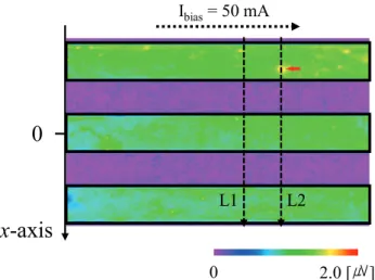
The three bridge sample analyzed by LTSLM with a bias current of 50 mA. Fig.2 shows the SLM image of the three bridge sample with a bias current of 50 mA at 90.5 K.

There is an inhomogeneous region on L2 which is indicated by a small red arrow in Fig. 2. It has larger voltage response compared to its neighbors.

Fig. 1. Temperature dependence of resistivity of samples with a bias current of 1 mA and a ramp rate of +1 K/min.

The one bridge sample has 𝑇

𝑐0

= 92.27 K and the three bridge sample has 𝑇

𝑐0

= 90.36 K.

Fig. 2. A SLM image of the three bridge sample with a bias current of 50 mA at 90.5 K. Two dotted arrows in the image indicate positions analyzed in detail. The small red arrow points out an inhomogeneous region on L2. The solid rectangles indicate the region of bridges.

Fig. 3. Distribution of 𝛿𝑉

max

and 𝑇

𝑐max

of the three bridge sample along L2 in Fig. 2. The dotted circle indicates the inhomogeneous region which pointed out by the small red arrow in Fig. 2.

To analyze the local critical temperature of 𝑇

𝑐max

in detail, we measured the maximum voltage signal 𝛿𝑉

max

along L1 and L2 in Fig. 2. We performed line scans at various temperatures in the superconducting transition region. 𝑇

𝑐max

at given positons are evaluated from a series of line scans. The 𝑇

_𝑐^max

is defined as the temperature at 𝛿𝑉

max

[23]. The standard deviation of 𝑇

𝑐max

is good indicator for the sample inhomogeneity. The distributions of 𝛿𝑉

max

and 𝑇

𝑐max

of L2 show in Fig. 3. The dotted circle in Fig. 3 points out the same inhomogeneous region in Fig.

2. The standard deviations of 𝑇

𝑐max

of L1 and L2 are 0.041 K and 0.043 K and the average values of 𝑇

𝑐max

are 90.411 K and 90.426 K, respectively. Although L2 still has relatively larger 𝛿𝑉

max

in the dotted circle region, L1 and L2 have similar standard deviation of 𝑇

𝑐max

and it indicates the three bridge sample is quietly homogeneous.

We measured the local magnetic field ℎ

𝑙

(𝑥, 𝑦) of samples in an applied external magnetic field by SHPM.

Fig. 4a and Fig.4b are SHPM images with 100 Oe of an

90.0 90.5 91.0 91.5 92.0 92.5 93.0 93.5 0

10 20 30 40 50 60 70 80 90

100 One bridge Three bridge I_bias : 1 mA Ramp rate : +1 K/min

Re sis tiv ity (µΩ cm)

Temperature (K)

L1 L2

2.0 [㎶]

0 I

_bias

= 50 mA

0 x-axis

-1000 -500 0 500 1000

0.0 0.2 0.4 0.6 0.8 1.0 1.2 1.4 1.6 1.8

T

maxc

(K)

δV_max

T ^max_c

x-axis position (µm) δV

max

(µ V)

90.30 90.32 90.34 90.36 90.38 90.40 90.42 90.44 90.46 90.48 90.50 90.52 90.54

26

(3)

Muyong Kim, Sangkook Park, Heeyeon Park, and Hyeong-Cheol Ri

external magnetic field at 81 K. As shown in Fig. 4a, the external magnetic field penetrated to the center of each sample and the distribution of ℎ

𝑙

(𝑥, 𝑦) is symmetric with respect to y-axis of both samples. We also carried out line scans in various applied fields along lines L3 and L4 in Fig.

5 for investigating local magnetic properties of samples.

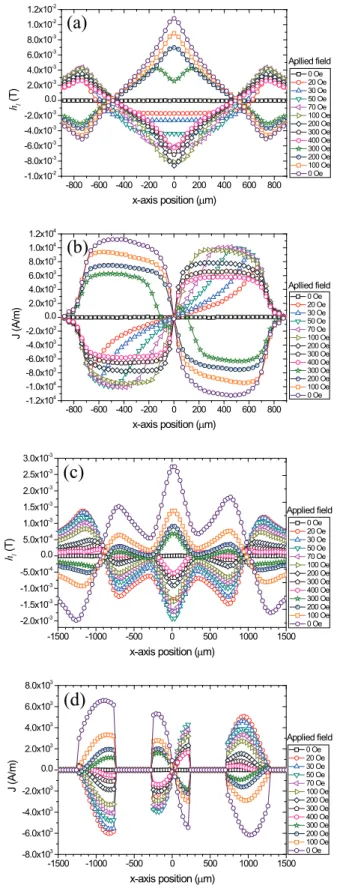
The one bridge sample was cooled to 81.0 K in zero magnetic field. Then the applied magnetic field increased from 0 Oe to 400 Oe and then reduced to 0 Oe while maintaining the temperature. The distributions of magnetic field of the one bridge sample in different external magnetic fields are shown in Fig. 5a. As the applied magnetic field increased from 0 Oe to 200 Oe, the magnetic field penetrates from the edge to the center of the sample. The local magnetic field which was fully penetrated has qualitatively the same shape up to 400 Oe.

And then during the external magnetic field reduced from 400 Oe to 0 Oe, the magnetic field distribution of the sample has reverse shape of previous one. This result is consistent with the Bean’s critical state model [1, 2].

Fig. 5b is the local current density which is calculated from the results of Fig. 5a using the inversion calculation method. In this case, the current density and the measured magnetic field has following relation [8].

(a) One bridge sample

(b) Three bridge sample

Fig. 4. Distribution of the stray magnetic field ℎ

𝑙

(𝑥, 𝑦) of (a) the one bridge sample and (b) the three bridge sample in 100 Oe of an external field at 81.0 K. The solid rectangles indicate the region of bridges.

Fig. 5. (a) Distribution of the magnetic field ℎ

_𝑙

(𝑥, 𝑦) of the one bridge in various applied field in L3 in Fig. 4a at 81 K, (b) the calculated local current density from (a) using the inversion calculation method. And (c) distribution of the magnetic field ℎ

_𝑙

(𝑥, 𝑦) of the three bridge in various applied field in L4 in Fig. 4b at 85 K, (d) the calculated local current density from (c) using the inversion calculation method.

-83.0 74.0 [Oe]

L3 0

x-axis

-44.5 45.0 [Oe]

L4 x-axis

0

-800 -600 -400 -200 0 200 400 600 800 -1.0x10^-2

-8.0x10^-3 -6.0x10^-3 -4.0x10^-3 -2.0x10^-3 0.0 2.0x10^-3 4.0x10^-3 6.0x10^-3 8.0x10^-3 1.0x10^-2 1.2x10^-2

Apllied field

hl (T)

x-axis position (µm)

0 Oe 20 Oe 30 Oe 50 Oe 70 Oe 100 Oe 200 Oe 300 Oe 400 Oe 300 Oe 200 Oe 100 Oe 0 Oe

(a)

-800 -600 -400 -200 0 200 400 600 800 -1.2x10⁴

-1.0x10⁴ -8.0x10³ -6.0x10³ -4.0x10³ -2.0x10³ 0.0 2.0x10³ 4.0x10³ 6.0x10³ 8.0x10³ 1.0x10⁴ 1.2x10⁴

J (A/m)

0 Oe 20 Oe 30 Oe 50 Oe 70 Oe 100 Oe 200 Oe 300 Oe 400 Oe 300 Oe 200 Oe 100 Oe 0 Oe Apllied field

(b)

-1500 -1000 -500 0 500 1000 1500

-2.0x10^-3 -1.5x10^-3 -1.0x10^-3 -5.0x10^-4 0.0 5.0x10^-4 1.0x10^-3 1.5x10^-3 2.0x10^-3 2.5x10^-3 3.0x10^-3

0 Oe 20 Oe 30 Oe 50 Oe 70 Oe 100 Oe 200 Oe 300 Oe 400 Oe 300 Oe 200 Oe 100 Oe 0 Oe Applied field

hl (T)

(c)

-1500 -1000 -500 0 500 1000 1500

-8.0x10³ -6.0x10³ -4.0x10³ -2.0x10³ 0.0 2.0x10³ 4.0x10³ 6.0x10³ 8.0x10³

J (A/m)

0 Oe 20 Oe 30 Oe 50 Oe 70 Oe 100 Oe 200 Oe 300 Oe 400 Oe 300 Oe 200 Oe 100 Oe 0 Oe Applied field

(d)

27

(4)

Analysis of the local superconducting properties in YBCO coated conductors with striations

𝜇

₀

𝐽(𝑛)

= � 𝑛 − 𝑛

^′

𝜋 �

1 − (−1)

^𝑛−𝑛^′

𝑒

^𝜋𝑑

𝑑

²

+ (𝑛 − 𝑛

^′

)

²

𝑛′

+ [𝑑

²

+ (𝑛 − 𝑛

^′

)

²

− 1]�1 + (−1)

^𝑛−𝑛^′

𝑒

^𝜋𝑑

� [𝑑

²

+ (𝑛 − 𝑛

^′

+ 1)

²

][𝑑

²

+ (𝑛 − 𝑛

^′

− 1)

²

] �

(2)

In Fig. 5a we can observe that the local screening current was generated from the edge of the sample and penetrated into the center during the magnetic field increased to 200 Oe. According to the Bean’s critical state model, the generated current density in the sample always has a magnitude of the critical current density [1, 2]. Fig. 5b shows that the maximum local current density is decreased by increasing external magnetic field. This feature can be understood well in terms of field dependence of critical current density [24]. As shown in Fig. 5a, at 𝐻

𝑓

= 200 Oe, the local magnetic field fully penetrated to the center of the sample. For 𝐻

app

≥ 𝐻

𝑓

, the local current density has the same value over the entire range of the sample. It corresponds to the condition that the critical current density is spatially constant in those regions.

We carried out similar experimental procedure on the three bridge sample. Likewise, the three bridge sample was cooled to 85.0 K in zero magnetic field. And then, the external magnetic field increased from 0 Oe to 400 Oe and reduced to 0 Oe while maintaining the temperature. Fig. 5c shows the distribution of the magnetic field of the three bridge sample. The three bridge sample has one inner bridge and two outer bridges. It is equivalent to that the one bridge sample was divided into three equal parts.

Therefore, the distribution of the magnetic field of the three bridge sample is qualitatively similar to the one bridge sample. In Fig. 5c, as the applied magnetic field increased from 0 Oe to 50 Oe, the magnetic field penetrates from the edge of outer bridges to the center of the inner bridge. The local magnetic field which was fully penetrated, during the external magnetic field reduced from 400 Oe to 0 Oe, the magnetic field distribution of the sample has reverse shape of previous one. The result of the distributions of the magnetic field of the three bridge sample is similar to the one bridge sample. Fig. 5d shows the distribution of the current density which is calculated from the results of Fig. 5c. The current density of the three

(a) (b)

(c) (d)

Fig. 6. (a)-(c) Local magnetization curves of the three bridge sample at 81.0 K. And (d) overlapping the distribution of the normalized remanent field from the second 0 Oe in Fig. 5c and the distribution of the normalized local hysteresis loss calculated from the local magnetization curves of P1-P9. There is schematic diagram of the measured positions of P1-P9 in (d).

P3 P5

-600 -400 -200 0 200 400 600

-6.0x10^-3 -4.0x10^-3 -2.0x10^-3 0.0 2.0x10^-3 4.0x10^-3 6.0x10^-3

hl (T)

H_app (Oe)

-600 -400 -200 0 200 400 600

-6.0x10^-3 -4.0x10^-3 -2.0x10^-3 0.0 2.0x10^-3 4.0x10^-3 6.0x10^-3

hl (T)

H_app (Oe)

P7

P1 P2 P3 P7 P8 P9 P5 P4

P6 x-axis

y-axis

-1500 -1000 -500 0 500 1000 1500

-0.8 -0.6 -0.4 -0.2 0.0 0.2 0.4 0.6 0.8 1.0

P9 P8 P6 P7

P5

P3 P4 P2 hl,rem (χ)

Normalized magnetizaion loss

x-axis position (µm) Normalized remanent field : hl,rem(χ) [a.u.]

P1 -0.8

-0.6 -0.4 -0.2 0.0 0.2 0.4 0.6 0.8 1.0 Normalized hysteresis loss [a.u.]

-600 -400 -200 0 200 400 600

-6.0x10^-3 -4.0x10^-3 -2.0x10^-3 0.0 2.0x10^-3 4.0x10^-3 6.0x10^-3

hl (T)

H_app (Oe)

28

(5)

Muyong Kim, Sangkook Park, Heeyeon Park, and Hyeong-Cheol Ri

bridge sample has different values over the cross section.

The overall shape of the distribution of the magnetic field of the three bridge sample was similar to the one bridge sample, but the distribution of the current density of the three bridge sample shows different pattern. This effect is caused by changing the geometry of the film.

We also investigated the local magnetization curves of 9 points of the three bridge sample using SHPM shown as Fig. 6d. The sample was cooled to 81.0 K in zero magnetic field. The hysteresis measurement was carried out for -500 Oe ≤ 𝐻

app

≤ 500 Oe. The results are shown in Fig. 6a-c.

The shapes of the hysteresis loops are symmetric about P5 which is the center of the sample. From the Bean’s critical state model, we can obtain an expression for hysteresis loss [24]

𝑄 = 1

𝜇

0

�2𝐻

max

𝐻

𝑓

− 4

3 𝐻

^𝑓²

� (3)

where 𝑄 is the hysteresis loss per unit volume, 𝐻

max

is the maximum applied magnetic field and 𝐻

𝑓

is the characteristic field when the fields are able to reach the center of the sample. If 𝛽 ≡ 𝐻

𝑓

/𝐻

max

and 𝛽 ≪ 1 , equation (3) approximately can be written as [25]

𝑄 ≅ 2𝐻

max

𝜇

₀

𝐻

_𝑓

(4)

In this case, 𝑄 is proportional to 𝐻

𝑓

. Equation (3) and equation (4) are defined on the whole sample. However, for local magnetic property measurement, we have to define the local hysteresis loss 𝑞 which can be defined as

𝑄 ≡ � 𝑞(𝑥)𝑑𝑥

^𝑎

−𝑎

(5)

where 𝑎 is the half width of the sample. Similarly as equation (4) using 𝑞 and ℎ

𝑓

, we can derive the following relation.

𝑞(𝑥) ≅ 2𝐻

max

𝜇

₀

𝑎 ℎ

^𝑓

(𝑥) (6)

It means that the local hysteresis loss is determined by the characteristic field as ℎ

𝑓

(𝑥). The distribution of ℎ

𝑓

(𝑥) is equal to the distribution of the maximum remanent field.

We can measure the maximum remanent field when the external magnetic field is zero by decreasing the external field from the maximum value. The magnitude of the maximum remanent field equals ℎ

𝑓

(𝑥) in same positon.

Fig. 6d shows comparison of the normalized remanent field and the normalized local hysteresis loss. We can see that they fits well each other. Although the Bean’s critical state model neglect the applied magnetic field dependence of the current density, it is still valid in our experiment as shown in Fig. 6d.

4. CONCLUSION

In this study, we prepared the YBCO coated conductors with striations. The one bridge sample has one filament and the three bridge sample has three filaments. We carried out LTSLHPM to investigate the local superconducting properties. The one bridge sample and the three bridge sample have the critical temperature 92.27 K and 90.36 K, respectively. The difference of the transition temperature 1.91 K might be caused by just different substrate of films, not their shape. However it only gives the information of the whole sample, not the local properties. LTSHPM allows us to investigate the local superconducting properties.

To analyze sample inhomogeneity of them, we used LTSLM visualizing the distribution of 𝛿𝑉 which is related to the distribution of 𝑇

𝑐max

. As the results, the standard deviation of 𝑇

𝑐max

is about 0.04 K. Although there are inhomogeneous region in L2 of Fig. 2, it has very small difference of the standard deviation about 0.002 K between L1 and L2. It gave that the sample has homogeneous distribution of 𝑇

_𝑐^max

.

The local magnetic field ℎ

𝑙

(𝑥, 𝑦) of the samples in applied magnetic fields was measured by SHPM. We take two lines from the local magnetic field ℎ

𝑙

(𝑥, 𝑦) and carried out line scans on those two lines in various applied magnetic field. The magnetic field penetrated starting from the edge to the center. It could be understood by the Bean’s critical state model. The shape of the distribution of the magnetic field looks similar. Using inversion calculation method, we obtained the distribution of the local current density. It shows that the local current density of the three bridge sample has different pattern with the one bridge, respectively. This effect is caused by changing the geometry of the film.

We also investigated the local magnetization curves of the three bridge sample. We could visualize the distribution of the local magnetization loss and compare with the distribution of the remanent field. Those two distributions fits each other. It could be demonstrated by the Bean’s critical state model. Although the Bean’s critical state model is theoretical model, its results are valid in the experimental results.

REFERENCES

[1] C. P. Bean, “Magnetization of hard superconductors,” Phys. Rev.

Lett., vol. 8, pp. 250-253, 1962.

[2] C. P. Bean, “Magnetization of high-field superconductors,” Rev.

Mod. Phys., vol. 36, pp. 31-39, 1964.

[3] H. P. Wiesinger, F. M. Sauerzopf and H. W. Weber, “On the calculation of Jc from magnetization measurements on superconductors,” Physica C, vol. 203, pp. 121-128, 1992.

[4] E. H. Brandt and M. V. Indenbom, “Type-II superconductor strip with current in a perpendicular magnetic field,” Phys. Rev. B, vol.

48, pp. 12_893-906, 1993.

[5] E. Zeldov, J. R. Clem, M. McElfresh and M. Darwin,

“Magnetization and transport currents in thin superconducting films,” Phys. Rev. B, vol. 49, pp. 9802-9822, 1994.

[6] T. Schuster, M. V. Indenbom, M. R. Koblischka, H. Kuhn and H.

Kronmuller, “Observation of current-discontinuity lines in type-II superconductors,” Phys. Rev. B, vol. 49, pp. 3443-3452, 1994.

29

(6)

Analysis of the local superconducting properties in YBCO coated conductors with striations

[7] E. H. Brandt, “Thin superconductors in a perpendicular magnetic ac field: General formulation and strip geometry,” Phys. Rev. B, vol.

49, pp. 9024-9040, 1994.

[8] Y. Mawatari, “Critical state of periodically arranged superconducting-strip lines in perpendicular fields,” Phys. Rev. B, vol. 54, pp. 13_215-221, 1996.

[9] T. H. Johansen, M. Baziljevich, H. Bratsberg, Y. Galperin, P. E.

Lindelof, Y. Shen and P. Vase, “Direct observation of the current distribution in thin superconducting strips using magneto-optic imaging,” Phys. Rev. B, vol. 54, pp. 16_264-269, 1996.

[10] M. Friesen and A. Gurevich, “Nonlinear current flow in superconductors with restricted geometries,” Phys. Rev. B, vol. 63, pp. 064521_1-26, 2001.

[11] J. Ogawa, S. Fukui, M. Yamaguchi, Takao Sato and O. Tsukamoto,

“Magnetization loss in a striated YBCO coated conductor considering the intrinsic critical current distribution,” IEEE Trans.

Appl. Supecond., vol. 16, no. 2, pp. 111–114, 2006.

[12] J. McDonald and J. R. Clem, “Theory of flux into thin films with field-dependent critical current,” Phys. Rev. B, vol. 53, 8643-8650, 1996.

[13] J. R. Clem and R. P. Huebener, “Application of low-temperature scanning electron microscopy to superconductors,” J. Appl. Phys.

vol. 51, pp. 2764-2773, 1980.

[14] R. Gross, M. Hartmann, K. Hipler, R. P. Huebener, F. Kober and D.

Koelle, “Spatial resolution limit for the investigation of high-Tc films by low temperature scanning electron microscopy,” IEEE Trans. Magn., vol.25, pp. 2250-2253, 1989.

[15] R. Gross and D. Koelle, “Low temperature scanning electron microscopy of superconducting thin films and Josephson junctions,”

Rep. Prog. Phys., vol. 57, pp. 651-741, 1994.

[16] N. Dieckmann, A. Bock and U. Merkt, “Spatially resolved analyses of epitaxial and electrical properties of YBa2Cu3O7 devices,” Appl.

Phys. Lett., vol. 68, pp. 3626-3628, 1996.

[17] D. Abraimov, A. G. Sivakov, A. V. Lukashenko, M. V. Fistul, P.

Muller and A. V. Ustinov, “Spatially resolved measurements of critical parameters in superconducting filaments by laser scanning technique,” IEEE Transa. Appl. Supercond., vol. 11, pp. 3170-3173, 2001.

[18] A. G. Sivakov, A. P. Zhuravel, O. G. Turutnov and I. M. Dmitrenko,

“Spatially resolved char- acterization of superconducting film and cryoelectronic devices by means of low temperature scanning laser microscope,” Appl. Surf. Sci., vol. 106, pp. 390-395, 1996.

[19] H. B. Wang, S. Guènon, J. Yuan, A. Iishi, S. Ariswa, T. Htano, T.

Yamashita, D. Koelle, and R. Kleiner, “Hot spots and waves in Bi2Sr2CaCu2O8 intrinsic Josephson junction stacks : A study by low temperature scanning laser microscopy,” Phy. Rev. Lett., vol.

102, pp. 017006, 2009.

[20] A. M. Chang, H. D. Hallen, L. Harriott, H. F. Hess, H. L. Kao, J.

Kwo, R. E. Miller, R. Wolfe, J. V. D. Ziel and T. Y. Chang,

“Scanning Hall probe microscopy,” Appl. Phys. Lett., vol. 61, pp.

1974-1976, 1992.

[21] D. Davidovic, S. Kumar, D. H. Reich, J. Siegel, S. B. Field, R. C.

Tiberio, R. Hey and K. Ploog, “Correlations and disorder in arrays of magnetically coupled superconducting rings,” Phys. Rev. Lett., vol. 76, pp. 815-818, 1996.

[22] Y. Abulafia, D. Giller, Y. Wolfus, A. Shaulov, Y. Yeshurun, D.

Majer, E. Zeldov, J. L. Peng and R. L. Greene, “Investigation of flux creep in high-Tc superconductors using Hall-sensor array,” J. Appl.

Phys., vol. 81, pp. 4944, 1997.

[23] S.K. Park, J.M. Kim, S.B. Lee, S.H. Kim, G. Y. Kim and H-C. Ri,

“Spatial distribution of the local resistive transition and the critical current density in YBCO coated conductors using low-temperature scanning laser microscopy,” Cryogenics, vol. 51, pp. 241–6, 2011.