Design Sensitivity Analysis and Topology Optimization of Thermal Systems Considering Convection Heat Transfer
Heegon Moon†, Semyung Wang* and Hokyung Shim**
대류를 고려한 열전달 시스템의 민감도 해석 및 위상 최적 설계
문희곤† · 왕세명* · 심호경**
Key Words : topology optimization(위상최적설계), convection(대류), heat transfer(열전달), sensitivity analysis(민감도 해석)
Abstract
This paper presents the adjoint variable design sensitivity analysis for thermal systems considering both conduction and convection heat transfer. Both nodal temperature and total heat flow are considered to be objective functions and design sensitivity formulas are derived for each case. For the case of convection heat transfer, the adjoint analysis is carefully proceeded to obtain a precise result. A topology optimization example is examined for a simple planar square plate in order to design a heat exchanger as verification.
1. INTRODUCTION
From the 1950s, numbers of researches have been done in optimization of thermal systems either analytically [1] or numerically. And much attention was paid for shape optimization from the 1980s [2-4].
Design sensitivity equations were well established for the linear and the nonlinear systems considering the conduction but not much for convection.
Topology optimization in thermal systems, however, is a relatively recent technique and is being done by some researchers. A topology optimization was presented for a heat conduction problem of minimum resistance between input and output points [5]. Furthermore, many researches have been done for coupled problems [6,7].
This paper presents the adjoint variable design sensitivity analysis (DSA) for thermal systems considering conduction and convection heat transfer.
For the convenience, finite element equations are provided in Chap.2. In Chap.3, DSA formulas and their derivation processes are given. Both nodal temperature
and total heat flow are considered to be objective. For the case of convection heat transfer, a special treatment is applied to the adjoint analysis to obtain a precise result. Equations for numerical implementation for topology optimization are given in Chap.4. Finally, as an example, a square plate is optimized in order to design a heat exchanger for verification purpose.
2. GOVERNING EQUATIONS
n Γ2
Γ1
qf
Γ3
( , )
h b
q h T
Ts
Figure 1. A thermal system with boundary conditions Consider a general heat transfer system including convection shown in Fig.1 then the governing equation can be written as
† 광주과학기술원 기전공학과 박사과정 E-mail : [email protected]
TEL : (062)970-2429 FAX : (062)970-2384 * 광주과학기술원 기전공학과 교수
** 광주과학기술원 기전공학과 박사과정
(k T r( )) q r r Rb( ) ; 3
−∇ • ∇ = ∈ (1)
and boundary conditions are
1 2
( ) 3 s
f f b h
T T on
k T q on
h T T qn on
= Γ
∂ = Γ
∂
− = Γ
(2)
where the coefficient k denotes the thermal conductivity(W/m·K), T temperature(K), qb internal heat generation rate per unit volume(W/m3), qf the external heat flux(W/m2), qh the convective heat flux(W/m2), hf the convection heat transfer coefficient(W/m2·K), and Tb temperature of coolant.
In order to take advantages of the Finite Element Method (FEM), variational procedures are applied to Eq.1 and 2. As a result, an algebraic equation is obtained for each finite element from the differential equation, that is,
[ ][ ]
( )
( )3
( ) ( )
2 3
( ) ( ) ( )
( ) ( ) ( )
( ) ( ) ( )
e
e
e e
e
e e e
c h
e T c
e T
h
e b f
b
e e e
b f h
K K K
K k N N d K hNN d
Q q N d q Nd hT Nd Q Q Q
Ω Γ
Ω Γ Γ
= +
= ∇ ∇ Ω
= Γ
= Ω + Γ + Γ
= + +
∫
∫
∫ ∫ ∫
(3)
In this equation, Kc( )e is a thermal conductivity matrix, Kh( )e a matrix representing the convection, N a shape function, Q( )e a load (heat flow) vector. Note that the convection coefficient appears on both the system matrix (K) and the load vector (Q), which makes special adjoint loads in the design sensitivity analysis. And the convection matrix Kh( )e is generally simplified as a diagonal matrix [8], that is,
( )3
( )( , ) e ( )
he
K i i hN i d
=∫Γ Γ (4)
where (i,i) and (i) represent the corresponding matrix and vector components respectively. Assembling every finite element, the global matrix equation is obtained as
K T =Q (5)
3. DESIGN SENSITIVITY ANALYSIS
Topology optimization is considered to be a heavy computational problem since it deals with thousands of design variables. An adjoint variable method (AVM) [9]
is probably the unique alternative to calculate sensitivity information in such a big size problem.
Consider a performance index form the thermal system as
( , ( ))b T b
ψ ψ= (6)
where b is a vector of design variables, then the corresponding adjoint equation to Eq.6 can be written as
K T
ψT λ ∂
= ∂ (7)
Finally, the gradient information is obtained by
T ( )
d Q KT
dbψ = ∂∂ψ λb + ∂∂b −∂∂b % (8)
where the tilde (~) indicates a variable that is to be held constant for of partial differentiation.
3.1 Nodal Temperature as a Performance Index When the temperature of the k-th nodal point is chosen as the performance index, that is,
1 u TT
ψ = (9)
where the u is the vector which has 1 in k-th position and 0 in elsewhere. Then the adjoint load will be
( )
1 u TT u
T T
∂ψ ∂
= =
∂ ∂ (10)
Before applying this load, the convection effect should be carefully considered because that the convection terms exist on both sides of the original equation (Eq.5). Applying the original convection load will add additional load or neglecting the convection heat will omit the system matrixKh. Thus, the convection coefficient is kept but the temperature of coolant Tb is set to 0 while performing the adjoint analysis.
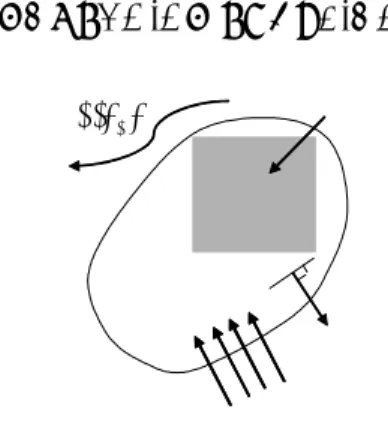
3.2 Input Heat Flow Rate as a Performance Index Another common performance index in thermal systems is the heat flow rate in many heat exchangers such as cooling fins [1]. Suppose a planar surface shown in Fig.2 in which and arbitrary heat flows to one end and the other ends are insulated and convection heat transfer occurs at the top surface.
Ts
f b, h T
Figure 2. A planar heat transfer system with convection occurs at the top surface
If the design goal is to obtain a maximum convection heat flow rate, owing to the energy conservation law, an equivalent problem is to find the maximum heat in-flow rate at the left edge. If we rewrite Eq.5 in a partitioned form as
11 12 1
21 22 s
K K T Q
K K T R
=
(11)
where unknown variables enclosed by are determined by ordinary matrix operations. The total heat in-flow rate to the system is then defined as
2 v RT
ψ = (12)
where the vector v is a summation operator, that is,
[1,1, ,1]
v =T L . Taking differentiation on Eq.11 with respect to the single design variable and rearranging terms yields,
[ 21 22][ ] [ ][ ]21 1
R′= K′ K′ T + K T′ (13)
Thus the design sensitivity equation is
[ ] 1
2 21 22 21 1
T T T
S
v R v K K T v K T ψ′ = ′= ′ ′ T + ′
(14)
And the other equation of differentiation is
11 1 ( 11 1 12 s )
K T′= − K T K T′ + ′ +Q′ (15) Taking pre-multiplication an arbitrary matrix λT(with
suitable matrix size) holds the equation, i.e.,
11 1 ( 11 1 12 )
TK T T K T K Ts TQ
λ ′= −λ ′ + ′ +λ ′(16)
By letting λTK11= v KT 21 and solving the equation
11 21T 12
K λ = K v = K v (17)
Finally, following equation is obtained to calculate design sensitivity.
[ ]
2
21 22 11 1 12
11 12 11 12
21 22 21 22
( )
0 0
T
T T s T
T T T T T
T T T
v R
v K K T K T K T Q
K K K K
v T T Q
K K K K
v K T Q
ψ
λ λ
λ λ
λ λ
′= ′
′ ′ ′ ′ ′
= − + +
′ ′ ′ ′
′
= ′ ′ − ′ ′ +
′ ′
= − +
(18)
4. TOPOLOGY OPTIMIZATION
For topology optimization of the thermal system, artificial variables ρi, actually design variables, are introduced to interpolate material properties such as,
3 0
, , 0
, , 0
0 1
(1 )
i
f t i f t i
f l i f l
k k
h h
h h
ρ
ρ ρ
ρ
=
= < ≤
= −
(19)
where k0 represents the original conductivity and
, , ,
f t f l
h h convection heat transfer coefficients for the top surface and side edges for each finite element, respectively and the subscripts 0 indicate their original values. For the conduction, it is quite clear that when ρi near 1 indicates material being exist and near 0 void. But considering the convection, if there exists material then convection heat transfer occurs at the top surface but not at the element edges. On the contrary, when a element is considered to be void then heat transfer occurs only at the side edges. Figure 3 illustrates the cases to be considered for explaining the convection. In the area A, where material exist all of the its adjacent neighbors, convection occurs only at the top surface, which can be
mathematically interpreted through Eq. 19 by letting
i 1
ρ = . For the area C, void everywhere, a question may arise that the convection does not affect for empty space.
But considering a network model, shown in Fig. 4, if a conduction resister is open, ρ =i 0, then there will be no heat flow to the isolated system. Thus the convection resisters in the isolated system cannot affect the heat flow but elements in transition area, area B, receives high attentions according to Eq.19.
A AA A
B B B B
C C C C
Figure 3. An illustrative model for explaining material interpolation for the convection
Ts
Tb
Ts
Tb Tb Tb Tb Tb
Tb Tb Tb Tb
Figure 4. A network model for explaining material interpolation for the convection
Since each design variable is assigned to a individual finite element, the design sensitivity can be written as
( ) ( )
( ) e e ( )
e T e
i i i i
d Q K T
dψ ψ λ
ρ ρ ρ ρ
∂ ∂ ∂
= ∂ + ∂ − ∂ (20)
And from Eq.4 and 5, the load vector is the form of
( )e b h( )e ( T [1,1,1,1]) Q =T K w Qw = (21) After taking differentiation, finally, the design sensitivity for each design is
( ) ( ) ( ) 2 ( ) ( ) ( )
0( ) 3 0
e T e e e T e e
h b i c
i i
d K T T K T
dψρ ψρ λ ρ λ
= ∂ + − −
∂
(22)
5. NUMERICAL EXAMPLES
A 2 dimensional cooling fin is examined as a verificational purpose. A 20 x 50 mm2 plate (Fig.2) is considered to have heat conditions such that
0.2, f 0.005, b 25 , S 300
k= h = T = °C T = °C. Knowing that a larger temperature differences ensures higher convection heat transfer rate, an optimization problem is drawn to have high temperature at the middle of the right side end and 50% volume constraint is imposed, that is,
. . 0.5
Maximize nodal temperature at the middle of the right end s t volume fraction<
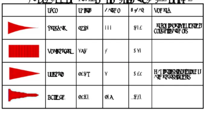
The optimal pattern is obtained after 34 iterations as shown in Fig.5(a) and the reanalysis model, Fig.5(b), is constructed for based on that pattern. Then the optimal design is compared to basic shapes[10] as shown in Table 1. From the table, the optimal model follows the analytical solution, the parabola shape, in terms of heat transfer rate per used volume.
(a) optimal topology
(a) reanalysis model
Figure 5. Topology optimization result for 2D fin design
Table 1. Comparison for effectiveness of fins
0.113 0.098 0.053 0.139 Q/Vol
432 48.93 Optimum
Most attractive in terms of manufacturing * 500
49.17 Triangle
1000 52.10 Rectangular
Largest heat dissipation per unit volume * 333
46.43 Parabola
Remark Volume
Total Q Type
0.113 0.098 0.053 0.139 Q/Vol
432 48.93 Optimum
Most attractive in terms of manufacturing * 500
49.17 Triangle
1000 52.10 Rectangular
Largest heat dissipation per unit volume * 333
46.43 Parabola
Remark Volume
Total Q Type
6. CONCLUSIONS
Design sensitivity analysis is presented using the adjoint variable method for the heat transfer system having a convective circumstance. Since convection phenomena affect both on the system matrix K and the load vector F an adjoint system proposed with care.
The input heat flow rate, an equivalent analogy to reaction force in structural systems, is examined as a performance index. Material interpolation function is provided to consider the conduction, convection at the top surface, and the side edges with a illustrative network model. As a verificational purpose, 2D fin is designed using the topology optimization method and it is shown that the optimal model matches fairly well with the analytical solution.
Acknowledgement
This research was supported by Center of Innovative Design Optimization Technology (ERC of Korea Science and Engineering Foundation).
References
[1] G. Ahmadi and A. Razani, “Some optimization problems related to cooling fins,” Int. J. Heat Mass Transfer, Vol. 16, pp.2369-2375, 1973
[2] K. Dems, “Sensitivity equations in thermal problems- II: Structural shape variation,” J. Thermal Stresses, Vol. 10, pp.1-16, 1987
[3] A. Sluzalec and M. Kleiber, “Shape sensitivity analysis for nonlinear steady-state heat conduction problems,” Int. J. Heat Mass Transfer, Vol. 32, No.
12, pp. 2609-2613, 1996
[4] R. Dziri and J. Zolesio, “Shape-sensitivity analysis for nonlinear heat convection,” Appl Math Optim, Vol. 35, pp.1-20, 1997
[5] M. Bendsoe and O. Sigmund, Topology Optimization – Theory, Methods and Applications, Springer,
pp.112, 2003
[6] O. Sigmund, “Topology optimization in multiphysics problems,” 7th AIAA/USAF/NASA/ISSMO Symposium on MAO, pp. 1492-1500, 1998
[7] L. Yin and G. Ananthasuresh, “A novel topology design scheme for the multi-physics problems of electro-thermally actuated compliant micro- mechanisms,” Sens. actuators. A Phys, Vol.97, No..2, pp. 599-609, 2002
[8] ANSYS Theory Reference, ANSYS Inc., ANSYS Ver [9] E.J. Haug, K.K. Choi, and V. Komkov, Design 7.0 Sensitivity Analysis of Structural Systems, Academic Press Inc., 1986
[10] F.P. Incropera and D.P. DeWitt, , Fundamentals of Heat and Mass Transfer, John Wiley & Sons, Inc., 1996