열전도 문제에 관한 위상 최적설계의 실험적 검증
차 송 현 1 ․김 현 석 1 ․조 선 호 1†
1서울대학교 아이소-지오메트릭 최적설계 창의연구단 및 조선해양공학과
Topology Design Optimization and Experimental Validation of Heat Conduction Problems
Song-Hyun Cha 1 , Hyun-Seok Kim 1 and Seonho Cho 1†
1
National Creative Research Initiatives(NCRI) Center for Isogeometric Optimal Design Department of Naval Architecture and Ocean Engineering.
Seoul National University, Seoul, 151-744, Korea
Abstract
In this paper, we verify the optimal topology design for heat conduction problems in steady stated which is obtained numerically using the adjoint design sensitivity analysis(DSA) method. In adjoint variable method(AVM), the already factorized system matrix is utilized to obtain the adjoint solution so that its computation cost is trivial for the sensitivity. For the topology optimization, the design variables are parameterized into normalized bulk material densities. The objective function and constraint are the thermal compliance of the structure and the allowable volume, respectively. For the experimental validation of the optimal topology design, we compare the results with those that have identical volume but designed intuitively using a thermal imaging camera. To manufacture the optimal design, we apply a simple numerical method to convert it into point cloud data and perform CAD modeling using commercial reverse engineering software. Based on the CAD model, we manufacture the optimal topology design by CNC.
Keywords : heat conduction, design sensitivity analysis, adjoint variable method, topology design optimization, experimental validation
†Corresponding author:
Tel: +82-2-880-7322; E-mail: [email protected] Received July 2 2014; Revised August 12 2014 Accepted August 13 2014
Ⓒ 2015 by Computational Structural Engineering Institute of Korea
This is an Open-Access article distributed under the terms of the Creative Commons Attribution Non-Commercial License(http://creativecommons.
org/licenses/by-nc/3.0) which permits unrestricted non-commercial use, distribution, and reproduction in any medium, provided the original work is properly cited.
1. Introduction
A topology design optimization method helps designers to find a suitable material layout for the required performances. Ever since Bendsøe and Kikuchi(1988) introduced the topology optimization using a homogenization method, many topology optimization methods have been developed for both linear and nonlinear structural problems(Cho and Jung, 2003). Since the topology optimization neces- sarily involves many design variables, gradient- based optimization methods are generally preferred.
Therefore, the sensitivity of performance measures
with respect to the design variables should be
determined in a very efficient way. Among various
DSA methods, a continuum-based adjoint variable
method(Choi et al., 1986) is known to be the most
efficient and accurate and widely used method in
topology optimization problems. In the continuum-
based DSA approach, the design sensitivity expre-
ssions are obtained by taking the first order variation
of the continuum variational equation. The continuum
DSA methods developed so far can handle several
types of design variables. The shape design sensi-
tivity for nonlinear transient thermal systems was
derived using Lagrange multiplier method(Tortorelli
Fig. 1 Body in space
et al., 1989a). Sluzalec and Kleiber(1996) employed the Kirchhoff transformation to derive the shape design sensitivity expressions for linearized heat con- duction problems using an adjoint variable approach.
Li et al.(1999) performed a shape and topology optimization of heat conduction problems using an evolutionary structural optimization method. Kim et al.(2010) developed an efficient DSA method using AVM for the non-shape problems like material property in the heat conduction problems at a steady state. In this paper, we experimentally verify the aforemen- tioned method by comparing the temperature variation of the optimal topology design and several different designs using a thermal imaging camera.
2. Heat conduction problems
Consider a body occupying an open domain in space that is bounded by a closed surface G as shown in Fig. 1. Material properties are assumed isotropic in domain . The boundaries are composed of a temperature boundary
, a flux boundary
, a convection boundary , and ∪ ∪ . Also, the boundaries are mutually disjointed. The body is subjected to the rate of internal heat generation Q and the following thermal boundary conditions. A prescribed temperature on
, a prescribed heat flux on
in the inward normal direction, and an ambient temperature ∞ on the convection boundary
are imposed. is an outward unit vector normal to the boundaries.
For a temperature field , a heat conduction equation in steady state is written as
(1)
where is a positive thermal conductivity corres- ponding to the principal axes and assumed to be independent of temperature. ∙ represents a partial derivative with respect to the i-coordinate.
The notation of repeated subscripts stands for the summation operation over the indices. Three kinds of boundary conditions are applied on the surface of the body as
on
(2)
on (3)
∞ on
(4)
where is a positive convection coefficient on the convection boundary. Space for the trial solution is defined as
∈ (5)
where denotes a Hilbert space of order one. Also, space for virtual temperature fields is defined as
∈ (6)
Using the virtual temperature field that satisfies homogeneous boundary conditions, a weak form of Equation (1) is written as
for all ∈ (7)
Note that Equation (7) implies the “principle of virtual power” and is independent of time since the steady state problems are considered. Integrating Equation (7) over a unit time leads to the “principle of virtual work” and yields an identical expression.
Thus, we regard Equation (7) as a principle of
virtual work hereafter. Using the boundary condi-
tions in Equations (2)~(4), Equation (7) can be
written as
(8)
∞ for all. ∈
Defining a bilinear thermal energy form
≡
(9)
and a linear load form
≡
∞ (10)
Equation (8) can be written as Find ∈ such that
for all ∈ (11)
3. Continuum-based design sensitivity analysis
3.1 Direct differentiation method
Consider a non-shape design variable vector that consists of the thermal conductivity of each element.
Fora given design , Equation (11) can be written as Find ∈ such that
for all ∈ (12)
where the subscript u indicates the dependence of the abstract form on the design variation. A variational equation corresponding to the perturbed design
is written as
for all ∈ (13)
Using Equation (13), the first order variations of each term in Equation (12) with respect to its explicit dependence on the design variable are defined as
′
(14)
′ ≡
(15)
where the ‘~’ denotes that the dependence on design variation is suppressed. Note that is independent of since it is an arbitrary virtual temperature field that belongs to .
Consider the solution of Equation (12). Define the first order variation of the solution with respect to the design as
′ ≡
lim
→
(16)
Using the chain rule of differentiation and the Equation (14), the following holds
(17)
′ ′
Using Equations (15) and (17) and taking the first order variation of Equation (12), we have
′ ′ ′ for all ∈ (18)
Next, consider a general performance functional that may be written, in an integral form, as
∇ ∇ (19)
Taking the first order variation of Equation (19), we have the following expression.
′
(20)
∇
∇
′ ∇ ∇ ′
′ ∇ ∇ ′
Once finding ′ from Equation (18), we trivially obtain the design sensitivity of performance measure from Equation (20).
3.2 Adjoint variable method
To define an adjoint equation for the heat conduc- tion problems, replace the implicit dependence terms
′ and ∇ ′ in Equation (20) by a virtual tempe- rature and equate the terms involving to the bilinear thermal energy form to yield the adjoint equation as
∇ ∇ (21)
∇ ∇
where the adjoint response satisfies the homoge- neous boundary condition. Since ∈ and ∈ , Equation (18) can be rewritten as
′ ′ ′ ∀ ∈ (22)
Noting that ′∈ and ∈ , Equation (21) can be rewritten as
′ ′ ∇ ∇ ′ (23)
′ ∇ ∇ ′
for all ′∈
Knowing that ∙∙ is a symmetric operator, the following holds.
′ ′ (24)
Equations (22) and (23) are equivalent and so we can write the following equation.
′ ∇ ∇ ′ (25)
′ ∇ ∇ ′ ′ ′
Substituting Equation (25) into (20), we have
′ ′ ′ (26)
To evaluate the Equation (26), we need not only the original response but also adjoint response . The efficiency and accuracy of Equation (26) will be demonstrated in section 5.
4. Topology Design Optimization
The objective of the topology optimization method is to find an optimal material distribution that mini- mizes the thermal energy stored in the system under prescribed thermal loadings. The material distribu- tion can be represented using a normalized bulk material density function that has a continuous variation from zero to one, taking the value of 1.0 for solid material and 0.0 for void. For the topology optimization using the finite element method, the structural domain is discretized into NE finite elements and the bulk material densities are assumed constant in each element. The design variable, bulk material density of each element, is associated with the thermal conductivity using the following expression as
(i=1,2,...,NE) (27)
≺ ≤ ≤ (28)
where is the thermal conductivity of original material. A penalty parameter P is used to enforce a concentrated distribution of material. The lower bound of material, , is introduced to avoid numerical singularity. A topology design optimization problem is stated as
Minimize
∞ (29)
Subject to ≤ (30)
where , , , ∞ , and are a temperature
field, a prescribed heat flux, a rate of internal heat generation, an ambient temperature, and an allowable volume, respectively.
For the topology optimization, it is very important to make the problem convex to obtain a unique optimal solution regardless of initial design. Otherwise, it may have many local minima and thus the optimal result depends on its initial design. If the Hessian of the unconstrained function that consists of the objective function and constraints is positive definite, the optimization problem is convex. In this topology optimization formulation, only linear constraints with respect to the design variables are considered so that the Hessian of the compliance functional affects the convexity of problem. To check the convexity of performance measure of Equation (29), consider the state equation that is equivalent to the Equation (11) as
(31)
where , , , , and are the bulk material density, an internal load, an external load, a system matrix, and a response vector, respectively. Taking the derivative of the state equation with respect to the response leads to
(32)
and with respect to the design variable yields
(33)
Taking the derivative of second equality in Equation (31) with respect to the design variable yields
(34)
where Equation (33) is used in the second equality.
The thermal compliance functional is rewritten in a
discretized form
(35)
Taking the derivative of the compliance functional with respect to the design variable , we have
(36)
where Equation (34) is used in the second equality.
Taking the derivative of Equation (36) with respect to the design variable again yields
(37)
The last term of Equation (37) is expressed using Equation (34) as
(38)
Thus, Equation (37) can be expressed in terms of the design variable as
(39)
where is the second order derivative of matrix with respect to design variable . If the penalty parameter is equal to zero or one, the second term in Equation (39) vanishes so that the problem is convex. Otherwise, it may have many local minima.
Since the topology optimization necessarily uses
many design variables, gradient-based optimization
methods are generally preferred. Therefore, the
Design Variable
FDM(a) AVM(b) (b)/(a)(%) -9.3845×10⁻³ -9.3856×10⁻³ 100.0117
-2.5933×10⁻³ -2.5936×10⁻³ 100.0116
-2.0694×10⁻³ -2.0696×10⁻³ 100.0097
-1.9682×10⁻³ -1.9684×10⁻³ 100.0102
-8.9883×10⁻⁴ -8.9894×10⁻³ 100.0122
Table 1 Comparison of design sensitivity Fig. 2 Rectangular plate
sensitivity of the performance measures with respect to the design variables should be determined in a very efficient manner. Among various DSA methods, the continuum-based adjoint variable method is known to be most efficient and accurate and thus widely used in topology optimization problems. To derive the adjoint design sensitivity, consider a thermal compliance functional
∇ ∇ (40)
Taking the first order variation of Equation (29) with respect to the design variables leads to
′ ′ ∇ ∇ ′ (41)
′ ∇ ∇ ′
′
′
∞ ′
Thus
′ (42)
The adjoint equation is written as
∇ ∇ (43)
∇ ∇
∞
Comparing Equation (43) with Equation (11), the following holds.
(44)
The compliance sensitivity using Equation (26) is obtained as
′ ′ ′ (45)
Using Equation (42), Equation (45) is reduced to
′ ′ ′ (46)
5. Numerical Examples
The first example is to verify the DSA method in the temperature field. Consider a rectangular plate (10cm by 5.5cm with thickness of 1.5mm) that consists of 14,080(88 by 160) finite elements with temperature and concentrated heat flux boundary conditions as shown in Fig. 2. Temperature boundary
0℃ is imposed at 10 elements each on top and bottom of the left side and a heat flux 133,333(W/m 2 ) is applied at 42 elements on the center of the right side. The thermal conductivity coefficient of aluminum 237(W/m․℃) is used in this problem. Design variables are the thermal conductivity coefficients of certain elements as shown in Fig. 2. Performance measure is the thermal compliance of the structure.
The obtained analytical sensitivity is compared with the finite difference one. In Table 1, the thermal compliance sensitivity with respect to the thermal conductivity of each element is shown. The last column shows the percent agreement between those.
Excellent agreements are observed.
Initial design(a) Final design(b) (b)/(a)(%) Objective function 92.8575 28.1253 30.2887
Table 2 Optimization result Fig. 3 Topology optimization result
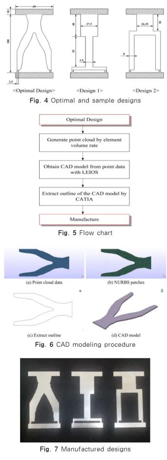
Fig. 4 Optimal and sample designs
Fig. 5 Flow chart
Fig. 6 CAD modeling procedure
Fig. 7 Manufactured designs
Consider the same structure in Fig. 2. This time,
the design variables are the thermal conductivity coefficients of all the elements. Performance measure is the thermal compliance of the structure, and allowable volume is 40% of the original one. The final material distribution after the topology optimization is shown in the Fig. 3. As shown in Table 2, the thermal compliance has been decreased to about 70%
of the initial one.
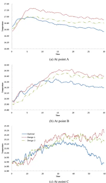
The purpose of topology optimization in heat conduction problems is to find an optimal material layout that yields a thermally stiff structure. To verify the topology optimization results we compare the temperature of the optimal design and two different models generated intuitively , design 1 and design 2, which have an identical volume as shown in Fig. 4. To measure the temperature, a thermal imaging camera VarioCAM head HiRes 640G is used which has 0.03 K thermal resolution. To impose a heat flux boundary condition, 133,333(W/m 2 ), we utilized a power supply to mainta 50V and 0.22A on a PTC heater. For the temperature boundary condition, 0℃, we used ice water.
Aluminum is used to manufacture the optimal and two different designs since fabrication is easy and it has sufficient thermal conductivity. The flow chart of manufacturing is shown in Fig. 5. First of all, by using a simple numerical scheme(Lee and Min, 2003), we convert the information of optimal design to point cloud data(Fig. 6(a)). Then we obtain the NURBS(Non Uniform Rational B-Spline) patch
model(Fig. 6(b)), by utilizing Leios 2010.1 3D3
Solutions. After that, we transform it into IGES file
format with CATIA v5 by Dassault Systems to get
Fig. 8 Temperature measuring points
Fig. 9 Temperature contours at each point
Fig. 10 Temperature variations at each point