using Adjoint Sensitivity Analysis Method
Kim, Min-Geun* Kim, Jae-Hyun** Cho, Seonho†
···
Abstract
In this paper, using an adjoint variable method, we develop a design sensitivity analysis(DSA) method applicable to heat conduction problems in steady state. Also, a topology design optimization method is developed using the developed DSA method.
Design sensitivity expressions with respect to the thermal conductivity are derived. Since the already factorized system matrix is utilized to obtain the adjoint solution, the cost for the sensitivity computation is trivial. For the topology design optimization, the design variables are parameterized into normalized bulk material densities. The objective function and constraint are the thermal compliance of structures and allowable material volume respectively. Through several numerical examples, the developed DSA method is verified to yield very accurate sensitivity results compared with finite difference ones, requiring less than 0.25% of CPU time for the finite differencing. Also, the topology optimization yields physical meaningful results.
Keywords : heat conduction, design sensitivity analysis, adjoint variable method, topology optimization
···
†책임저자, 정회원․서울대학교 조선해양공학과/RIMSE 교수 Tel: 02-880-7322 ; Fax: 02-888-9298
E-mail: [email protected]
* 서울대학교 아이소-지오메트릭 창의연구단 연구원
** 서울대학교 조선해양공학과 학사과정
∙이 논문에 대한 토론을 2011년 2월 28일까지 본 학회에 보내주시 면 2011년 4월호에 그 결과를 게재하겠습니다.
1. Introduction
A topology design optimization method helps designers to find a suitable material layout for the required performances. Ever since Bendsøe and Kikuchi (1988) introduced the topology optimization using a homogenization method, many topology optimization methods have been developed for both linear and nonlinear structural problems (Cho and Jung, 2003).
Since the topology optimization necessarily involves many design variables, gradient-based optimization methods are generally preferred. Therefore, the sensi- tivity of performance measures with respect to the design variables should be determined in a very efficient way. Among various DSA methods, a continuum-based adjoint variable method (Choi et al., 1986) is known to be most efficient and accurate and widely used in the topology optimization problems.
In the continuum-based DSA approach, the design sensitivity expressions are obtained by taking the
first order variation of continuum variational equation.
The continuum DSA methods developed so far can handle several types of design variables. In this paper, a continuum method for the non-shape problems like material property is considered. We develop an efficient DSA method for the heat conduction problems in steady state.
The shape design sensitivity for nonlinear transient thermal systems was derived using the Lagrange multiplier method (Tortorelli et al., 1989a) and the adjoint method (Tortorelli et al., 1989b). Sluzalec and Kleiber (1996) employed the Kirchhoff transformation to derive the shape design sensitivity expressions for the linearized heat conduction problems using an adjoint variable approach. Li et al. (1999) performed a shape and topology optimization of heat conduction problems using evolutionary structural optimization methods.
In section 2, the governing equation and weak formulation for the steady state heat conduction
Fig.1 Heat conduction problem
problems are discussed. In section 3, a continuum- based DSA method is formulated using both the direct differentiation method and the adjoint variable approach in a continuum form. In section 4, for the heat conduction problems, we formulate a topology optimization method where the developed DSA method is applied. In section 5, numerical examples are demonstrated to verify the accuracy of the developed analytical DSA method using the finite difference sensitivity and discuss the efficiency of the developed method. The topology design optimiza- tion is performed for several cases, which shows very reasonable results in physical point of view.
2. Heat conduction problems
Consider a body occupying an open domain in space that is bounded by a closed surface as shown in Fig. 1.
Material properties are assumed to be isotropic in domain . The boundaries are composed of a temperature boundary
, a flux boundary
, a convection boundary
, and ∪∪ . Also, the boundaries are mutually disjointed. The body is subjected to the rate of internal heat generation Q and the following thermal boundary conditions. A prescribed temperature on
, a prescribed heat flux on in the inward normal direction, and an ambient temperature ∞ on the convection boundary
are imposed. is an outward unit vector normal to the boundaries. For a temperature field , a heat conduction equation in steady state is written as
(1)
where is a positive thermal conductivity corres- ponding to the principal axes and assumed inde- pendent of temperature. ∙ represents a partial derivative with respect to i-coordinate .The notation of repeated subscripts stands for the summation operation over the indices. Three kinds of boundary conditions are imposed on the surface of body as
(2)
(3)
and
∞ (4)
where is a positive convection coefficient on the convection boundary. The space for the trial solution is defined by
∈
(5)where denotes a Hilbert space of order one.
Also, the space for the virtual temperature fields is defined by
∈
(6)Using the virtual temperature field that satisfies homogeneous boundary conditions, the weak form of Equation (1) is written by
for all ∈ (7)Note that Equation (7) implies the “principle of virtual power” and is independent of time since the steady state problems are considered. Integrating Equation (7) over a unit time leads to the “principle of virtual work” and yields an identical expression.
Thus, we regard the Equation (7) as a principle of virtual work hereafter. Using the boundary conditions in the Equations (2)~(4), the Equation (7) can be written as
∞
for all. ∈ (8)
Defining a bilinear thermal energy form
≡
(9)
and a linear load form
≡
∞ (10)
Equation (8) can be written as Find ∈ such that
for all ∈ (11)3. Continuum design sensitivity analysis
3.1. Direct differentiation method
Consider a non-shape design variable vector that consists of the thermal conductivity of each element. For the given design , Equation (11) can be written as
Find ∈ such that
for all ∈ (12)where the subscript indicates the dependence of the abstract form on the design variation. For a perturbation parameter , the variational equation corresponding to the perturbed design is written as
for all ∈ (13)Using the Equation (13), the first order variations of each term in Equation (12) with respect to its explicit dependence on the design variable are defined as
′
(14)and
′
≡
(15)where the ‘~’ denotes that the dependence on design variation is suppressed. Note that is independent of since it is an arbitrary virtual temperature field that belongs to .
Consider the solution of Equation (12). Define the first order variation of the solution with respect to the design as
′ ≡
lim
→
(16)
Using the chain rule of differentiation and the Equation (14), the following holds
′
′
(17)Using the Equations (15) and (17) and taking the first order variation of Equation (12), we have the following.
′
′
′
for all ∈ (18)Next, consider a general performance functional that may be written, in integral form, as
∇
∇ (19)Taking the first order variation of Equation (19), we have the following expression.
′
∇
∇
′ ∇∇′
′ ∇∇′
(20)Once finding ′ from Equation (18), we trivially obtain the design sensitivity of performance measure from Equation (20).
3.2. Adjoint variable method
To define an adjoint equation for the heat conduction problems, replace the implicit dependence terms ′ and ∇′ in Equation (20) by a virtual temperature and equate the terms involving to the bilinear thermal energy form
to yield the adjoint equation as
∇∇
∇∇
for all ∈ (21)
where the adjoint response satisfies the homo- geneous boundary condition. Since ∈ and ∈ , Equation (18) can be rewritten as
′′′ for all ∈ (22)
Noting that ′∈ and ∈ , Equation (21) can be rewritten as
′
′ ∇∇′
′ ∇∇′
for all ′∈ (23)
Knowing that ∙∙ is a symmetric operator, the following holds.
′′ (24)
Equations (22) and (23) are equivalent so that we can write the following equation.
′ ∇∇′
′ ∇∇′
′′ (25)Substituting Equation (25) into Equation (20), we have the following.
′
′′(26)To evaluate the Equation (26), we need not only the original response but also adjoint response . The efficiency and accuracy of Equation (26) will be demonstrated in section 5.
4. Topology Design Optimization
The objective of topology optimization is to find an optimal material distribution that minimizes the thermal energy stored in a system under prescribed thermal loadings. The material distribution can be represented using a normalized bulk material density function that has a continuous variation from zero to one, taking the value of 1.0 for solid material and 0.0 for void. For the topology optimization using the finite element method, the structural domain is discretized into NE finite elements and the bulk material densities are assumed constant in each element. The design variable, bulk material density of each element, is associated with the thermal conductivity using the following expression as
(i=1,2,...,NE) (27)
≺ ≤ ≤ (28)
where is the thermal conductivity of original material. A penalty parameter P is used to enforce a concentrated distribution of material. The lower bound of material, , is introduced to avoid numerical singularity. A topology design optimization problem is stated as
Minimize
∞ (29)
Subject to
≤ (30)where , , , ∞, and are a temperature field, a prescribed heat flux, a rate of internal heat generation, an ambient temperature, and an allowable volume, respectively.
For topology design optimization, it is very important to make the problem convex to obtain a unique optimal solution regardless of initial design. Otherwise, it may have many local minima and thus the optimal result depends on its initial design. If the Hessian of the unconstrained function that consists of the objective function and constraints is positive definite, the optimization problem is convex. In this topology optimization formulation, only linear constraints with respect to the design variables are considered so that the Hessian of the compliance functional affects the convexity of problem. To check the convexity of performance measure of (29), consider the state equation that is equivalent to the Equation (11) as
(31)
where , , , , and are the bulk material density, an internal load, an external load, a system matrix, and a response vector, respectively. Taking derivative of the state equation with respect to the response leads to
(32)
and with respect to the design variable yields
(33)
Taking the derivative of the second equality in the Equation (31) with respect to the design variable yields
(34)
where Equation (33) is used in the second equality.
The thermal compliance functional is rewritten in
the form of discretized form by
(35)
Taking the derivative of the compliance functional with respect to the design variable , we have
(36)where Equation (34) is used in the second equality.
Taking the derivative of the Equation (36) with respect to the design variable again yields
(37)The last term of Equation (37) is expressed, using Equation (34), as
(38)Thus, Equation (37) can be expressed in terms of the design variable as
(39)
where is the second order derivative of system matrix with respect to the design variable . If the penalty parameter is equal to zero or one, the second term in Equation (39) vanishes so that the problem is convex. Otherwise, it may have many local minima.
Since the topology optimization necessarily uses many design variables, gradient-based optimization methods are generally preferred. Therefore, the sensitivity of the performance measures with respect
Fig. 2 Square plate
Fig. 3 Design sensitivity to the design variables should be determined in a
very efficient manner. Among various DSA methods, the continuum-based adjoint variable method is known to be most efficient and accurate and thus widely used in the topology optimization problems.
To derive the adjoint design sensitivity, consider a thermal compliance functional
∇
∇ (40)
Taking the first order variation of Equation (29) with respect to the design variables leads to
′
′ ∇∇′
′ ∇∇′
′
′
∞′ (41)
Thus
′
(42)The adjoint equation is written as
∇∇
∇∇
∞ (43)
Comparing Equation (43) with Equation (11), the following holds.
(44)
The compliance sensitivity using Equation (26) is obtained as
′
′′ (45)
Using Equations (42), Equation (45) is reduced to
′ ′
′ (46)5. Numerical examples
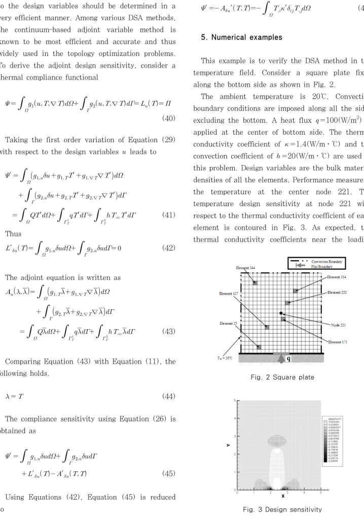
This example is to verify the DSA method in the temperature field. Consider a square plate fixed along the bottom side as shown in Fig. 2.
The ambient temperature is 20℃. Convection boundary conditions are imposed along all the sides excluding the bottom. A heat flux 100(W/m2) is applied at the center of bottom side. The thermal conductivity coefficient of 1.4(W/m․℃) and the convection coefficient of 20(W/m․℃) are used in this problem. Design variables are the bulk material densities of all the elements. Performance measure is the temperature at the center node 221. The temperature design sensitivity at node 221 with respect to the thermal conductivity coefficient of each element is contoured in Fig. 3. As expected, the thermal conductivity coefficients near the loading
Design
Variable i
T κ d d221
i
T κ Δ
Δ 221 (%)
d d221 221
i i
T T
κ κ Δ Δ
-7.89047043×10⁻³ -7.89057786×10⁻³ 100.00136
-8.28900388×10⁻⁴ -8.28913800×10⁻⁴ 100.00162
2.75000803×10⁻² 2.75004899×10⁻² 100.00149
-8.21570461×10⁻³ -8.21582671×10⁻³ 100.00149
-2.33197840×10⁻³ -2.33201285×10⁻³ 100.00148
-7.20091450×10⁻⁴ -7.20101849×10⁻³ 100.00144 Table 1 Comparison of design sensitivity
CPU time (seconds)
FDM DDM (DDM/FDM %) AVM (AVM/FDM %) 40.4882192 14.27052(35.246%) 0.100144(0.247%)
Table 2 Comparison of CPU time
Fig. 4 Topology design for various heat generation rates points turn out to be the most sensitive.
The obtained analytical sensitivity is compared with the finite difference sensitivity. In Table 1, the temperature sensitivity at node 221 with respect to the thermal conductivity of each element () is compared. stands for the analytical sensitivity using either the direct differentiation method (DDM) or the adjoint variable method (AVM). Those methods yield an identical result. ∆∆ represents the central finite difference sensitivity. The last column shows the percent agreement between the finite difference and the analytical sensitivities. Excellent agreements are observed.
In Table 2, the CPU costs required for the compu- tation of design sensitivity are summarized. We notice that only 0.1 second is required for the AVM and 14.3 seconds for the DDM whereas 40.5 seconds for the FDM. In general, the DDM requires appro- ximately 35% of CPU time for the FDM. However, the AVM does only 0.25% of CPU time for the FDM.
Comparing the DDM and AVM, the AVM just requires approximately 0.7% of CPU time for the DDM.
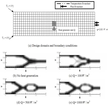
The next example is for the topology optimization under heat loading and temperature boundary using the derived design sensitivity. A rectangular model is subjected to a concentrated heat flux, temperature boundary, and an internal heat generation. The final material distribution after the topology optimization is also shown in the Fig. 4.
In Fig. 4, as the rate of internal heat generation
increases, significantly different topology results are obtained. As the magnitude of heat generation rate increases, we observe the complicated connectivity appearing (c). When Q increases (d), significantly different results are found. Further increase of heat generation rate results in a similar result (e).
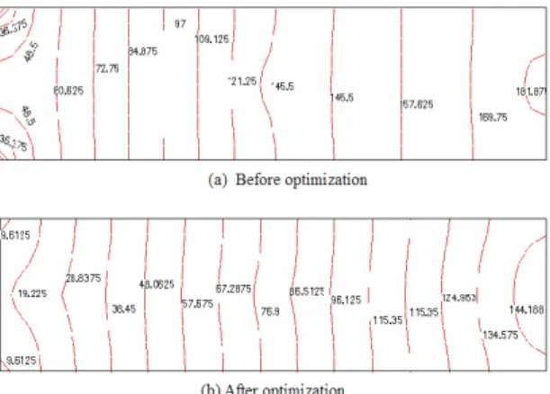
The purpose of topology optimization in heat conduction problems is to find an optimal material layout that yields thermally stiff structure. In other words, we want to find the layout hard to increase the temperature in the system for the given loading and boundary conditions. To investigate the effect of the topology optimization, we compare the temperature distributions in two cases. The one has uniformly distributed material property whose magnitude is reduced by 30 % of original one, (a) in Fig. 5. The other is the one obtained after the topology optimiza- tion, (b) in Fig. 5. It also uses 30 % of the original material and has the optimal material distribution.
In Fig. 5, in case the rate of internal heat generation Q is equal to 1000W/m3, temperature distributions in two models are compared. As expected, the optimal model (b) yields lower temperature distribution thro- ughout the whole domain. The temperature distribu- tions are approximately 34.33℃~194.03℃ for the model (a) and 9.61℃~153.80℃ for the model (b).
Fig. 5 Temperature comparison
Fig. 6 Three-dimensional problem
(a) 200W/m3
(b) 100W/m3
Fig. 7 Three-dimensional problem
(a) 200W/m3
(b) 100W/m3
Fig. 8 Single convection boundary problem The last example is an application of the developed
method to a three-dimensional problem. The model is subjected to temperature boundary and convection boundary conditions as shown in Fig. 6.
The objective of this example is to perform general topology optimization for three-dimensional problem and to verify the physical meaning of optimal topology. The model is composed of solid elements and the ambient temperature is 0℃. Temperature boundary conditions are imposed 0℃ at 4 nodes at bottom corners. The heat generation Q is applied in all elements. The objective function and constraint are the thermal compliance and the allowable material volume of 30%, respectively. In Fig. 7, the optimal material distributions are contoured as the heat generation Q decreases. The ambient tempera- tures of top surface and 3 slots are ∞
20℃, ∞
0℃, respectively.
In Fig. 8, in case single convection boundary of top surface is imposed, the optimal material distribu- tions are contoured as the heat generation decreases. The ambient temperatures of top surface is ∞ 20℃.
6. Conclusions
We have derived a weak formulation for heat conduction problems in steady state and a continuum- based DSA method using both a direct differentiation
and an adjoint variable approach in continuum form.
Also, a topology design optimization method for heat conduction problems has been developed using the adjoint DSA method. Since the already factorized system matrix is utilized in the adjoint variable method, the computing cost is significantly reduced.
For the topology design optimization, design variables are parameterized using bulk material densities.
Through several numerical examples, we verify the accuracy of the analytical DSA method using the finite difference sensitivity. The analytical DSA method yields very accurate sensitivity results compared with the central finite differencing. Comparing the efficiency of developed method, it just requires less than 0.3% of CPU time necessary for the finite differencing. Also, the topology optimization yields physically meaningful results. It could result in different topologies depending on the ratio of flux and internal heat generation rate. Comparing the tem- perature distributions before and after the topology optimization, significantly reduced temperature is observed.
Acknowledgement
This research was supported by Basic Science Research Program through the National Research Foundation of Korea (NRF) funded by the Ministry of Education, Science and Technology (Grant Number 2010-18282). The support is gratefully acknowledged.
References
Bendsøe, M.P., Kikuchi, N. (1988) Generating
Optimal Topologies in Structural Design using a Homogenization Method, Computer Methods in Applied Mechanics and Engineering, 71, pp.197∼
224.
Cho, S., Jung, H. (2003) Design Sensitivity Analysis and Topology Optimization of Displacement-Loaded Nonlinear Structures, Computer Methods in Applied Mechanics and Engineering, 192, pp.2539∼2553.
Haug, E.J., Choi, K.K., Komkov, V. (1986) Esign Sensitivity Analysis of Structural Systems, Academic Press, NewYork, pp.83~109.
Tortorelli, D.A., Haber, R.B., Lu, S.C-Y. (1989a) Design Sensitivity Analysis for Nonlinear Thermal Systems, Computer Methods in Applied Mechanics and Engineering, 77, pp.61∼77.
Tortorelli, D.A., Haber, R.B. (1989b) First-order Design Sensitivity Analysis for Transient Conduction Problems by an Adjoint Method, International Journal for Numerical Methods in Engineering, 28, pp.733∼752.
Sluzalec, A., Kleiber, M. (1996) Shape Sensitivity Analysis for Nonlinear Steady-State Heat Conduction Problems, International Journal for Numerical Methods in Engineering, 39, pp.2609∼2613.
Li, Q., Steven, Querin, S.O.M., Xie, Y.M. (1999) Shape and Topology Design for Heat Conduction by Evolutionary Structural Optimization, International Journal of Heat and Mass Transfer, 42, pp.3361∼
3371.
논문접수일 2010년 10월 29일
논문심사일 2010년 11월 4일
게재확정일 2010년 11월 29일