Optimal thresholds criteria for ROC surfaces

Optimal thresholds criteria for ROC surfaces

C. S. Hong ¹ · E. S. Jung ²

12 Department of Statistics, Sungkyunkwan University

Received 20 August 2013, revised 23 September 2013, accepted 1 October 2013

Abstract

Consider the ROC surface which is a generalization of the ROC curve for three−class diagnostic problems. In this work, we propose five criteria for the three−class ROC sur- face by extending the Youden index, the sum of sensitivity and specificity, the maximum vertical distance, the amended closest-to-(0,1) and the true rate. It may be concluded that these five criteria can be expressed as a function of two Kolmogorov−Smirnov statistics. A paired optimal thresholds could be obtained simultaneously from the ROC surface. It is found that the paired optimal thresholds selected from the ROC surface are equivalent to the two optimal thresholds found from the two ROC curves.

Keywords: Accuracy, classification, cut-off, marker, sensitivity, threshold, true rate.

1. Introduction

Roc curves are commonly used for the evaluation of diagnostic markers in two-class diag- nostic testing. For discrimination tasks with more than two events, it is necessary that the proper analysis of multiple-class diagnostic testing requires a generalization of ROC analy- sis. Recently, ROC analysis has been extended to three-class diagnostic problems (Scurfield, 1996; Mossman, 1999; Dreiseitl et al., 2000; Heckerling, 2001; Fawcett, 2003; Nakas et al., 2004, 2010; Patel and Markey, 2005; Wandishin and Mullen, 2009; and many others).

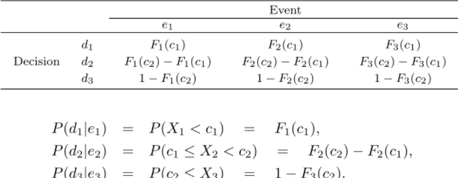
Consider a discrimination task involving three events, denoted {e 1 , e 2 , e 3 } as assigned by the testing procedure, in which an observer attempts to discriminate among a set of three decisions, denoted {d 1 , d 2 , d 3 }. Let {X 11 , X 12 , . . . , X 1n

} be a random sample of size n 1 obtained from the first class with the cumulative distribution function F 1 (·), and let {X 21 , X 22 , . . . , X 2n

} and {X 31 , X 32 , . . . , X 3n

} be random samples of sizes n 2 and n 3 ob- tained from the second and third classes, F 2 (·) and F 3 (·), respectively. Assume that F 1 (x) ≥ F 2 (x) ≥ F 3 (x) for all x. For two ordered thresholds (decision markers, cut−off point) c 1 ≤ c 2 , the following decision rule may be applied:

If X ≤ c ₁ then decision is class 1 (d ₁ ).

Else if c 1 ≤ X < c 2 then decision is class 2 (d 2 ).

Else decision is class 3 (d ₃ ).

1

Corresponding author: Professor, Department of Statistics, Sungkyunkwan University, Seoul 110-745, Korea. E-mail:[email protected]

2

Graduate student, Department of Statistics, Sungkyunkwan University, Seoul 110-745, Korea.

Table 1.1 shows the event-decision matrix of the observer. Each entry in the matrix speci- fies the probability that the observer will make a particular decision given that a particular event occurred. For example, the three probabilities, P (d k |e k ) (k = 1, 2, 3) are the true clas- sification rates, and the six probabilities, P (d i |e j ), (i 6= j) are the false classification rates.

Note that

Table 1.1 Event-decision probability matrix Event

e

e

e

d

P (d

|e

) P (d

|e

) P (d

|e

) Decision d

P (d

|e

) P (d

|e

) P (d

|e

) d

P (d

|e

) P (d

|e

) P (d

|e

)

Table 1.2 Event-decision distribution function matrix Event

e

e

e

d

F

(c

) F

(c

) F

(c

)

Decision d

F

(c

) − F

(c

) F

(c

) − F

(c

) F

(c

) − F

(c

) d

1 − F

(c

) 1 − F

(c

) 1 − F

(c

)

P (d 1 |e 1 ) = P (X 1 < c 1 ) = F 1 (c 1 ),

P (d ₂ |e 2 ) = P (c ₁ ≤ X 2 < c ₂ ) = F ₂ (c ₂ ) − F ₂ (c ₁ ), P (d 3 |e 3 ) = P (c 2 ≤ X 3 ) = 1 − F 3 (c 2 ).

Table 1.2 shows that the probabilities, P (d i |e j ), in Table 1.1 are represented by three cumulative distribution functions F j (·) and two thresholds c 1 ≤ c 2 .

The surface generated by the three kinds of the true classification rates as the two thresh- olds vary over the domain of X is called the ROC surface. The functional form of the ROC surface is

ROC s (p 1 , p 3 ) = F 2 (F ₃ ⁻¹ (1 − p 3 )) − F 2 (F ₁ ⁻¹ (p 1 )), 0 ≤ p 1 , p 3 ≤ 1,

where p ₁ = P (d ₁ |e ₁ ) and p ₃ = P (d ₃ |e ₃ ). The ROC surface is constructed by plotting the points (F ₁ (c ₁ ), F ₂ (c ₂ ) − F ₂ (c ₁ ), 1 − F ₃ (c ₂ )) in three dimensional unit−length cube (Nakas and Yiannoutsos., 2004).

Threshold selection in a three-class ROC surface has been explained in a theoretical con- text in He and Frey (2006). Nakas et al. (2010, 2013) generalized the Youden index for the three-class classification problem. In this paper, we extend the generalization of the Youden index and propose several optimal threshold criteria for a three−dimensional ROC surface.

There are four optimal threshold criteria which are related to the Youden index for the

ROC curve: the sum of the sensitivity and specificity, the maximum vertical distance, the

amended closest-to-(0,1), and the true rate. These four criteria defined on the ROC curve

are extended and developed for the ROC surface in Section 2. In Section 3, some examples

are illustrated to describe the relation between the paired thresholds obtained from the ROC

surface and the two thresholds obtained separately from the two ROC curves. We derive a

conclusion in Section 4.

2. Optimal criteria for the ROC surface

There are many criteria used to select optimal thresholds (Youden, 1950; Connell and Koepsell, 1985; Perkins and Schisterman, 2006; Kraznowski and Hand, 2009; Velez et al., 2007; Hong, 2009; and many others). Among them, the well-known Youden index J is defined as the maximum of the simple average of the differences between the true classification rate and the false classification rate for each event, that is, the average of F 1 (x) − (1 − F 1 (x)) and (1 − F 2 (x)) − F 2 (x). Hence the Youden index is represented as J = max[F 1 (x) − F 2 (x)]

(Youden, 1950), which is essentially the Kolmogorov−Smirnov statistic.

Consider four optimal criteria for the ROC curve which have a relationship with the Youden index: the sum of the sensitivity and specificity is defined to maximize the sum- mation of the sensitivity and the specificity, which is represented as SSS = max[F ₁ (x) + (1 − F ₂ (x))] (Connell and Koepsell, 1985). The MVD (maximum vertical distance) is de- fined as the maximum vertical difference between the ROC curve and the chance line:

M V D = max |ROC(p) − p| = max[F ₁ (x) − F ₂ (x)], where ROC(p) = F ₁ (F ₂ ⁻¹ (p)), p ∈ [0, 1]

(Kraznowski and Hand, 2009). The amended closest-to-(0,1) criteria, AC, is defined to min- imize the proportion of the smaller radius (r 2 ) (the distance between point (1, 0) and a point on the ROC curve) to the larger radius (r 1 )(the distance between point (0, 1) and the chance line), that is, AC = min[1 − F 1 (x) + F 2 (x)] (Perkins and Schisterman, 2006). And the balanced accuracy (BA) or the true rate (TR) is defined as the maximum of the arith- metic mean of the sensitivity (true positive rate) and the specificity (true negative rate):

T R = max [F 1 (x) + (1 − F 2 (x))]/2 (Velez et al., 2007; Hong, 2009). Hong and Joo (2010), Hong et al. (2010) and Yoo and Hong (2011) found that these five criteria are represented as a function of the Kolmogorov−Smirnov statistic. Hence we make use of these statistics for selecting a paired optimal thresholds based on the ROC surface.

First, Nakas et al. (2013) generalized the Youden index to multiple-class classification problems. However, to keep the definition of the Youden index for the ROC curve and extend its use to the three− class ROC surface, we will define a Youden index (J ₃ ) for the ROC surface which maximize the average of the three differences between the one true classification rate and the two false classification rates. And explain that the Youden index for the ROC surface has a relationship with Youden indices and KS statistics for the two ROC curves.

Proposition 2.1 Youden index for ROC surface J 3 = max

x,y;x<y [{F 1 (x) − (F 1 (y) − F 1 (x)) − (1 − F 1 (y))} + {(F 2 (y) − F 2 (x))

−(F 2 (x)) − (1 − F ₂ (y))} + {(1 − F ₃ (y)) − F ₃ (x) − (F ₃ (y) − F ₃ (x))}]/3

= max

x,y;x<y [2 × F 1 (x) + 2 × (F 2 (y) − F 2 (x)) + 2 × (1 − F 3 (y))]/3.

Corollary 2.1 Relation of J and KS

J 3 = 2/3 × (max[J 12 ] + max[J 23 ]) − 1/3

= 2/3 × (KS ₁₂ + KS ₂₃ ) − 1/3,

where J _ij is the Youden index for the two dimensional ROC curve consisting of F _i (·) and

F _j (·), and KS _ij is the Kolmogorov-Smirnov statistic for testing H ₀ : F _i (·) = F _j (·). That is,

J ₁₂ = max[F ₁ (x) − F ₂ (x)] for all x. And there exists constant, c ₁ , which satisfies F ₁ (c ₁ ) − F ₂ (c ₁ ) = max[F ₁ (x) − F ₂ (x)] for all x, denoted as KS ₁₂ .

By extending the sum of the sensitivity and specificity (SSS) to the three−dimensional ROC surface, we define ST R 3 to maximize the sum of the three true classification rates and its relationship as follows:

Proposition 2.2 Sum of three true rates for ROC surface ST R 3 = max

x,y;x<y [F 1 (x) + (F 2 (y) − F 2 (x)) + (1 − F 3 (y))].

Corollary 2.2 Relation of SSS and KS

ST R 3 = SSS 12 + SSS 23 − 1

= KS ₂₃ + KS ₁₂ + 1,

where SSS _ij is the SSS for the ROC curve consisting of F _i (·) and F _j (·).

The M V D (maximum vertical distance) for the ROC curve can be extended to a three−class ROC surface as the maximum vertical difference between the ROC surface, ROC 3 (p 1 , p 3 ), and the chance plane, g(p 1 , p 3 ) = 1-p 1 -p 3 .

Proposition 2.3 MVD for ROC surface M V D 3 = max

x,y;x<y [F 2 (F ₃ ⁻¹ (1 − p 3 )) − F 2 (F ₁ ⁻¹ (p 1 )) − (1 − p 1 − p 3 )]

= max

x,y;x<y [F ₂ (y) − F ₃ (y) + F ₁ (x) − F ₂ (x)].

Corollary 2.3 Relation of M V D and KS

M V D 3 = M V D 12 + M V D 23

= KS 23 + KS 12 ,

where M V D ij is the M V D for ROC curve consisting of F i (·) and F j (·).

The amended closest-to-(0,1) criteria can be extended to the amended closest-to-(1,1,1) criteria for the ROC Surface as min[pr ² ₂ /r ₁ ² ], where r ₁ ² and r ₂ ² are obtained as

r ₁ = p{(1 − F 1 (x)) ² + (1 − (F 2 (y) − F 2 (x))) ² + (F 3 (y)) ² } 1 − (F 1 (x) − F 2 (x) + F 2 (y) − F 3 (y)) , r ₂ = p{(1 − F ₁ (x)) ² + (1 − (F ₂ (y) − F ₂ (x))) ² + (F ₃ (y)) ² }.

Hence the amended closest-to-(1,1,1) criteria, AC 3 , can be defined as Proposition 2.4 Amended closest−to−(1,1,1) criteria for ROC surface

AC ₃ = min[

q r ₂ ² /r ² ₁ ]

= min[1 − (F 1 (x) − F 2 (x) + F 2 (y) − F 3 (y)).

Corollary 2.4 Relation of AC and KS

AC 3 = AC 12 + AC 23 − 1

= 1 − (KS 12 + KS 23 ),

where AC _ij is the amended closest-to-(0,1) for the ROC curve consisting of F _i (·) and F _j (·).

The balanced accuracy (BA) or the true rate (TR) can be generalized to the ROC surface as the maximum of the simple mean of the three kinds of true classification rates:

Proposition 2.5 T R for ROC surface T R 3 = max

x,y;x<y [1/3 × [F 1 (x) + (F 2 (y) − F 2 (x)) + (1 − F 3 (y))].

Corollary 2.5 Relation of T R and KS

T R ₃ = 2/3(T R ₂₃ + T R ₁₂ + 1/2)

= 1/3(KS 12 + KS 23 + 1),

where the T R _ij is the true rate for the ROC curve consisting of F _i (·) and F _j (·).

Therefore the five classification criteria such as J ₃ , ST R ₃ , M V D ₃ , AC ₃ and T R ₃ for the ROC surface are proposed and defined. And it is found that these five criteria for the ROC surface have relationship with the corresponding criteria for the ROC curves as well as the Kolmogorov-Smirnov statistics.

3. Three examples for the ROC surfaces

We consider three examples. The first and second examples were obtained from Scurfield (1996), and Nakas and Yiannoustsos (2004), respectively. And the final example was taken from other distributions. These examples are based on the normal distributions summarized in Table 3.1.

Table 3.1 Distribution functions of examples

Example F

(·) F

(·) F

(·)

1. N (−1, 1) N (0, 1.4

) N (1, 1.2

)

2. N (0, 1) N (1, 1.1

) N (1.4, 1.3

)

3. N (0, 1) N (1, 0.8

) N (2, 1.2

)

Table 3.2 Criteria for ROC curves

Example Threshold KS J SSS MVD AC TR

-0.2 0.3449 0.3449 1.3449 0.3449 0.6551 0.6725

1. 0.3 0.3050 0.3050 1.3050 0.3050 0.6816 0.6525

0.6 0.3677 0.3677 1.3677 0.3677 0.6323 0.6838

2. 1.7 0.1465 0.1465 1.1465 0.1465 0.8535 0.5732

0.4 0.4288 0.4288 1.4288 0.4288 0.5712 0.7144

3. 1.7 0.4079 0.4079 1.4079 0.4079 0.5921 0.7040

The results of Example 1 in Table 3.2 show that the values of KS, J , SSS, M V D, and T R for two distributions F ₁ and F ₂ were larger than those for F ₂ and F ₃ . On the other hand, AC for F 1 and F 2 had smaller value than for F 2 and F 3 , since AC attained the minimum value.

Hence, the classification power for F 1 and F 2 was greater than for F 2 and F 3 . Examples 2 and 3 can be explained in a similar manner. Table 3.2 shows the optimal thresholds for F 1

and F 2 in Examples 1 to 3 were -0.2, 0.6 and 0.4. And the optimal thresholds for F 2 and F 3

in the three Examples were 0.3, 1.7 and 1.7. These thresholds were obtained based on the two dimensional ROC curves.

Table 3.3 Criteria for ROC surface

Example Threshold J

ST R

M V D

AC

T R

1. -0.2 0.1000 1.6499 0.6499 0.3501 0.5500

0.3

2. 0.6 0.0094 1.5142 0.5142 0.4858 0.5047

1.7

3. 0.4 0.2245 1.8367 0.8367 0.1633 0.6122

1.7

Table 3.3 shows three paired thresholds and values of the five optimal criteria proposed in Section 2 for the ROC surface. It is easy to find that the paired optimal thresholds in Table 3.3 are identical to those in Table 3.2. Also we found there are relationships between these values in Table 3.2 and 3.3 using the five corollaries in Section 2. Among five optimal criteria in Table 3.3, all values for Example 3 were larger than those for Examples 1 and 2.

This means that the classification power for F 1 , F 2 and F 3 in Example 3 was greater than in Examples 1 and 2. This phenomenon could be derived from Figure 3.1.

Figure 3.1 demonstrates the three ROC surfaces corresponding to Example 1 to 3. From the ROC surfaces, we can understand the analytical interpretations discussed above. On each ROC surface, there is a mark which indicates the point corresponding to two optimal thresholds, ROC _s (p ₁ , p ₃ ) = {F ₂ (F ₃ ⁻¹ (1−p ₃ ))−F ₂ (F ₁ ⁻¹ (p ₁ ))}. The optimal threshold’s mark of Example 3 locates higher and more closer to (1, 1, 1) point than other marks of Example 1 and 2. Threrfore based on values of five optimal criteria and the corresponding marks on the ROC surface, the classification power of Example 3 is greater than other examples.

Figure 3.1 ROC surface

Table 3.4 contains three event−decision probability matrices of Example 1 to 3. For Exam- ple 1, the first and third true classification rates are high, and only the first true classification rate is high for Example 2. However, all three kinds of the true classification rates have higher values more than 0.5 in Example 3. Hence, we might conclude that Example 3 have the most classification power than Example 1 and 2 based on the results of Table 3.2, 3.3, 3.4 and Figure 3.1.

Table 3.4 Event-decision probability matrix

Ex 1 : Event Ex 2 : Event Ex 3 : Event

Decision e

e

e

e

e

e

e

e

e

d

0.7881 0.4432 0.1587 0.7257 0.3581 0.2692 0.6554 0.2266 0.0912 d

0.1150 0.1416 0.1212 0.2297 0.3797 0.3221 0.3000 0.5826 0.3101 d

0.0968 0.4152 0.7202 0.0446 0.2623 0.4087 0.0446 0.1908 0.5987

4. Conclusion

The five classification criteria J , SSS, M V D, AC and T R for the two-dimensional ROC curve were extended to the three-class ROC surface. Since these criteria have a relationship to the Kolmogorov-Smirnov statistic, it was found that the criteria for the ROC surface can be represented by the paired Kolmogorov−Smirnov statistics to test both F ₁ , F ₂ and F ₂ , F ₃ .

By using the five suggested classification criteria for the ROC surface, the paired optimal thresholds could be obtained. It was concluded that the paired optimal thresholds found from the ROC surface were identical to the two optimal thresholds selected from the two ROC curves.

In this paper, we assume only three events and decisions for a discrimination task. For more than three classes, the ROC analysis cannot be explained further. However for K (≥ 4) events and decisions, some optimal classification criteria might be extended and generalized.

In particular, criteria such as KS, J , SSS, M V D, AC and T R could be developed for K- class classification problems. With these classification criteria, K − 1 optimal thresholds are obtained with ease, since the optimal thresholds from the ROC surface are equivalent to the optimal thresholds obtained from the ROC curves. Therefore, this work provides a framework for further research.

References

Connell, F. A. and Koepsell, T. D. (1985). Measures of gain in certainty from a diagnostic test. American Journal of Epidemiology, 121, 744-753.

Dreiseitl, S., Ohno-Machado, L. and Binder, M. (2000). Comparing three-class diagnostic tests by three-way ROC analysis. Medical Decision Making, 20, 323-331.

Fawcett, T. (2003). ROC graphs: notes and practical considerations for data mining researchers, Technical report HPL-2003-4, HP Laboratories, 1-28.

He, X. and Frey, E. C. (2006). Three-class ROC analysis - The equal error utility assumption and the optimality of three-class ROC surface using the ideal observer. IEEE Transactions on Medical Imaging, 25, 979-986.

Heckerling, P. S. (2001). Parametric three-way receiver operating characteristic surface analysis using math-

ematica. Medical Decision Making, 21, 409-417.

Hong, C. S. (2009). Optimal threshold from ROC and CAP curves. Communications in Statistics-Simulation and Computation, 38, 2060-2072.

Hong, C. S. and Joo, J. S. (2010). Optimal thresholds from non-normal mixture. The Korean Journal of Applied Statistics, 23, 943-953.

Hong, C. S., Joo, J. S. and Choi, J. S. (2010). Optimal thresholds from mixture distributions. Journal of Korean Statistical Society, 23, 13-28.

Krzanowski, W. J. and Hand, D. J. (2009). ROC curves for continuous data, Chapman and Hall, London.

Mossman, D. (1999). Three-way ROCs. Medical Decision Making, 19, 78-89.

Nakas, C. T. and Yiannoutsos, C. T. (2004). Ordered multiple-class ROC analysis with continuous mea- surements. Statistics in Medicine, 23, 3437-3449.

Nakas, C. T., Alonzo, T. A. and Yiannoutsos, C. T. (2010). Accuracy and cut-off point selection in three- class classification problems using a generalization of the Youden index. Statistics in Medicine, 29, 2946-2955.

Nakas, C. T., Dalrymple-Alford, J. C., Anderson, T. J. and Alonzo, T. A. (2013). Generalization of Youden index for multiple-class classification problems applied to the assessment of externally validated cogni- tion in Parkinson disease screening. Statistics in Medicine, 32, 995-1003.

Patel, A. C. and Markey, M. K. (2005). Comparison of three-class classification performance metrics: A case study in breast cancer CAD. International Society for Optical Engineering, 5749, 581-589.

Perkins, N. J. and Schisterman, E. F. (2006). The inconsistency of “optimal” cutpoints obtained using two criteria based on the receiver operating characteristic curve. American Journal of Epidemiology, 163, 670-675.

Scurfield, B. K. (1996). Multiple-event forced-choice tasks in the theory of signal detectability. Journal of Mathematical Psychology, 40, 253-269.

Velez, D. R., White, B. C., Motsinger, A. A., Bush, W. S., Ritchie, M. D., Williams, S. M. and Moore, J. H.

(2007). A balanced accuracy function for epistasis modeling in imbalanced datasets using multifactor dimensionality reduction. Genetic Epidemiology, 31, 306-315.

Wandishin, M. S. and Mullen, S. J. (2009). Multiclass ROC analysis. Weather and Forecasting, 24, 530-547.

Yoo, H. S. and Hong, C. S. (2011). Optimal criterion of classication accuracy measures for normal mixture.

Communications for Statistical Applications and Methods, 18, 343-355.

Youden, W. J. (1950). Index for rating diagnostic test. Cancer, 3, 32-35.