1. INTRODUCTION
A significant attention has been focused on SMAs over the recent years, especially in the development of innovative engineering systems such as smart materials, active absorbers, micro actuators, etc. Unlike other alloys, SMAs possess peculiar characteristics such as a pseudo-elasticity and shape memory effects (SME), and many application areas have arisen since its discovery. Pseudo-elasticity has been successfully applied in medical and non-medical fields; for example, dental arches, catheter guide wires, vascular stents, eyeglass frames, mobile phone antennas, brassier wires, etc. The SME application area is limited compared to the field of pseudo-elasticity. SME has been applied to pipe couplings or fasteners, headings of thermostats, valves, and actuators of micro-robots; however, applications to precise engineering systems are somewhat problematic due to the highly nonlinear dynamic behavior of this alloy.
Examples of hard nonlinearities include backlash-like hysteresis and a saturation due to SME, which causes difficulties for a precise control. Thus, numerous approaches for an SMA actuator control have been proposed. However, some unsolved problems still remain. Ordinary PID control schemes often show the steady-state errors and the limit-cycle problems. Majima et al. [1] proposed a control system composed of a PID feedback loop and a feedforward loop. They showed that the limit-cycle oscillations were significantly reduced and the tracking control performances were improved. Grant and Hayward [2] applied a variable structure control scheme to a pair of antagonist actuators and realized a smooth and robust control. Kumagai et al. [3] applied a neuro-fuzzy based control to SMA actuators, but tracking was not so accurate. D. Grant [4] developed a disk-type SMA actuator with a rapid response of about 2.0 Hz and applied the relay control that was robust against the parameter variations of the actuator. Hasegawa and Majima [5] tried to compensate for the hysteresis of SMAs using an inverse hysteresis model for an SMA plant; however, a generalized model that accurately explains the behavior of an SMA is difficult to obtain. Further, it is also difficult to
achieve a perfect compensation even though a generalized model is obtained.
On the other hand, the TDC does not require an exact mathematical model and also provides a robustness against variations of a systems’ parameters and disturbances. The key concept of the TDC is the use of time delay information to estimate the total plant nonlinearities. The TDC has been applied in many important plants such as robot systems [6-7] and a magnetic bearing [8]. In these applications, the TDC provided highly satisfactory results even under large system parameter variations and disturbances. We have also studied that application of the TDC to an SMA actuator in other literatures [9-10]. Based on the previous study on the TDC, we developed the SMCTE scheme, which is the modified version of the sliding mode control (SMC) to alleviate the requirement of a detail mathematical model.
As well as the contribution of the above control methodology, the model identification for SMA actuators has also been studied. Most easily and most commonly used constitutive model for SMAs is the Liang’s model but it is not adequate to simulate the dynamic behavior of SMA actuators due to its numerical fault at the change of the phase transformation. Therefore, the dynamics for an SMA actuator was newly derived using the modified Liang’s model. The derived dynamics showed a continuity at the change of the phase transformation process but the original Liang’s model could not. SMA actuator characteristics could be described well by using this dynamics. For the prediction of the control performance and gain tuning of the TDC, the derived dynamics was superbly used.
2. NEWLY DERIVED DYNAMICS
FOR THE SMA ACTUATOR
2.1 Governing equationWe consider the dynamics of the rotational motion and bias-type actuator as shown in Fig. 1. In a bias-type actuator, the SMA actuator can be shrunk by a thermal excitation and can be restored to its original shape by a bias spring force under cooling conditions. In Fig. 1, θ denotes the rotary
The Sliding Mode Control with a Time Delay Estimation (SMCTE)
for an SMA Actuator
Hyo Jik Lee
*, Ji Sup Yoon
**and Jung Ju Lee
**** Division of Spent Fuel Technology Development, Korea Atomic Energy Research Institute, Daejeon, Korea (Tel : +82-42-868-4866; E-mail: [email protected])
** Division of Spent Fuel Technology Development, Korea Atomic Energy Research Institute, Daejeon, Korea (Tel : +82-42-868-2855; E-mail: [email protected])
*** Department of Mechanical Engineering, Korea Advanced Institute of Science and Technology, Daejeon, Korea (Tel : +82-42-869-3033; E-mail: [email protected])
Abstract: We deal with the sliding mode control using the time delay estimation. The time delay estimation is able to weaken the
need for obtaining a quantitative plant model analogous to the real plant so the sliding mode control with a time delay estimation (SMCTE) is very suitable for plant such as SMA actuators whose quantitative model is difficult to obtain. We have already studied the application of the time delay control (TDC) to SMA actuators in other literature. Based on the previous study on the TDC, we developed the gain tuning method for the SMCTE, which results were nearly the same as the TDC. With respect to the step response, the SMCTE proved its predominance in a comparison with other control schemes such as the PID control and the relay control. As well as the contribution of the above control methodology, the model identification for SMA actuators has also been studied. The dynamics for an SMA actuator was newly derived using the modified Liang’s model. The derived dynamics showed a continuity at the change of the phase transformation process but the original Liang’s model could not.
angle of the moment of inertia, J and R is the radius of the pulley coupled with the angle sensor. In most of the literature, including reference [1], the thermal term in the constitutive equation is not considered; however, in this paper the thermal term is included as the following equation:
T E B AR
P&= θ&+ ξ&+ & (1)
where P is the force developed by the SMA actuator, ξ is the martensite fraction, T is the temperature and the dotted means a time derivative. Detail description of Eq. (1) and a derivation of the final form of dynamics were explained at length in reference [10]. The final form of the dynamics of the SMA actuator can be written as follows:
) ( ) ( 1 ) )( 1 ( ) ( ) ( 2 i i i i T T E BC BD R BD ABD A K R J − + − − = − − + + + − + −θ ρθ θ θ θ
θ&& && & & (2)
where subscript i represents the initial value and the upper
bar means the average value between time
i
t and t.
Fig. 1 Structure of the SMA actuator.
2.2 Modified Liang’s model
We modified the original Liang’s model in terms of the phase diagram and discontinuity. Original Liang’s model is not sufficient to illustrate the behavior of SMAs under various temperature and stress conditions. Therefore, we added more constrained conditions as follows:
))) 0 ( ) 0 (( )) 0 ( ) 0 ( ) (( )) 0 ( ) 0 ( ) 0 ((( ) ( ) ( ))) 0 ( ) 0 (( )) 0 ( ) 0 ( ) (( )) 0 ( ) 0 ( ) 0 ((( ) ( ) ( σ σ σ σ σ σ σ σ σ σ σ σ d and dT or d and dT and dT d C or d and dT and C dT d and M T C M T C M A if d and dT or d and dT and dT d C or d and dT and C dT d and A T C A T C A M if M M f M s M A A s A f A ≤ ≤ ≤ < ≤ ≤ ≤ ≤ ≤ − ≤ ≤ − → ≤ < ≤ ≤ ≤ ≤ < ≤ ≤ − ≤ ≤ − → (3)
Each process, possesses three more constraints related to directions as well as the phase transformation band as shown in Fig. 2.
2.3 Verification of the derived dynamics
In order to verify the derived dynamics of the SMA actuator, we have solved the implicit differential equation, Eq.
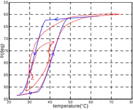
(2), iteratively. In respect to the phase transformation process, we have used a prediction-correction algorithm. In the prediction step, we essentially extrapolate the state variables from the previous point to the new point. In the correction step, we find the point where the phase transformation process changes within the current step using the bisection method. Subsequently, the current step is divided into two steps having different phase transformation processes. We have implemented the verification of the derived dynamics with a 0.05 sec fixed step size using the Runge-Kutta solver of SIMULINK/MATLAB. First, we compared the major hysteresis in the simulation with the result in the experiment as shown in Fig. 3. In this case, we used the material properties of [10].
Fig. 2 Phase diagram of the modified Liang’s model.
20 30 40 50 60 70 80 55 60 65 70 75 80 85 90 95 temperature(°C) θ( deg )
Fig. 3 Hysteresis curves. Dashed line: experiment; solid line: simulation.
The modified Liang’s model is valuable when an incomplete cyclic hysteresis occurs as shown in Fig. 4. The temperature sequence in Fig. 4 develops an incomplete phase transformation so the path lay inside the major hysteresis. It is very important to notice that the modified Liang’s model maintains a continuous martensite fraction at the change of the phase transformation but the original model cannot.
3. Sliding mode control with a time delay estimation
3.1 Problem of SMCAs mentioned above, the dynamics of an SMA actuator has a large parameter variation as well as an unknown parameter, so it is difficult to obtain the nominal part of the system. This drawback is a crucial problem in SMC, because SMC requires the nominal model of the system. However, SMC with a time delay estimation need not obtain the nominal part. This advantage will be used in the systems which model cannot be obtained or which model is difficult to obtain.
3.2 SMCTE derivation
We consider the following nonlinear equation:
u B H d u X X B X X B X X f X X f x ˆ ) ( )] ; , , ( ) ; , , ( [ ) ; , , ( ) ; , , ( 1 1 1 1 ) ( + = + ∆ + + ∆ + = t t t t t m m m m n L L L L (4) where x x xni T ni i m i i i i [ , , , ] , 1, , ) 1 ( L L & ∈ℜ = = − X is the state
sub-vector, which forms the global state vector ; , , 1 , , , ] , , , [ 1 2 r 1n xi i m m i i r T m T T L LX ∈ℜ =
∑
= = X X . ] , , , [ ; ] , , , [ ; ] , , , [ ; , , 1 , , ] [ , ] [ ; ] , , , [ , ] , , , [ ) ( ) ( 2 ) ( 1 ) ( 2 1 2 1 1 1 1 1 2 1 n T m m n n n m T m m T m m m ij m m ij m T m m T m m x x x u u u d d d m j i b b f f f f f f ℜ ∈ = ℜ ∈ = ℜ ∈ = = ℜ ∈ ∆ = ∆ ℜ ∈ = ℜ ∈ ∆ ∆ ∆ = ∆ ℜ ∈ = × × L L L L L L x u d B B f fu denotes the input vector and corresponds to ∆T in the rotary-type SMA actuator; f denotes nonlinear function, which may be unknown, yet bounded; B denotes the control distribution matrix; Bˆ denotes the nominal control distribution matrix; d the denotes disturbances; H denotes the total uncertainty.
The control input vector of the SMCTE can be calculated as follows: ] ) ( ) sgn( [ ˆ ) ( ] ) sgn( [ ˆ ) ( ) ( 1 ) ( 1 α x x s K Ps B u H x α s K Ps B u − − − + − − + − = − + − − − = − − L t L t n n d est n d (5) where ); ( ˆ ) ( ) (t L (n) t L t L est=H − =x − −Bu − H
[
1, ,]
, >0; =diag p L pm pi P[
1, ,]
, >0; =diagk Lkm ki K[
sgn( ), ,sgn( )]
; ) sgn( 1 T m s s L = s . 0 1 ) sgn( , 0 0 ) sgn( , 0 1 ) sgn(si = if si> si = if si= si =− if si< For the estimation of the total uncertaintyest
H , we
borrowed the time delay estimation from the time delay control. Consequently, the unknown total uncertainty at the present can be simply calculated using the past information at
L
t− if L is enough small. For the sliding hyperplanes, the definition of s is as follows:
∫
+ = (e(n) α)dt s (6) where [ , ( ), ( )] , ( ) ( ) ( ); 2 ) ( 1 ) ( 1 2 m i i ni di n i n i m T n m n n n x x e e e e ∈ℜ = − = L e∑
− = = = ℜ ∈ = 1 1 ) ( , 2 1, , , ] , , 1, , . [ ni k k i k i i m T m e i Lm Lα α λ α α αEach element of the right side vector of Eq. (6) should be selected as a Hurwitz polynomial of the tracking errors of the associated state sub-vector. Substituting Eq. (5) for Eq. (4), we obtain the following s-dynamics:
est H H s K Ps s&=− − sgn()+ − (7)
Eq. (7) is the constant plus proportional rate reaching law. Using Lyapunov stability criterion Kcan be simply obtained. For the system of Eq. (4) to be stable, the condition s &Ts≤0 should be satisfied. Therefore, K should satisfy the following inequality: m i i est ii ( ) , 1, , ) (K ≥ H−H = L (8)
Due to the switching term of Eq. (5), the SMCTE cannot avoid a chattering problem like SMC. The switching action term can be replaced with a continuous term by making a boundary layer neighboring the sliding hyperplanes as follows: ] ) ( ) ( [ ˆ L) -( B 1 Ps K Φ1s x( ) x() α u u= + − − − − + − − − L t sat t n n d (9) where
{
1, , 1}
, 0; 1 1= Φ− Φ− Φ > − i m diag L Φ . 1 ) ( , 1 ) sgn( ) (a = a if a > sata =aif a≤ sat 3.3 SMCTE implementationLet us consider a single input system with a one state sub-vector. Without a loss of generality the control input can be expressed as: ⎥ ⎦ ⎤ ⎢ ⎣ ⎡ ⎟⎟ ⎠ ⎞ ⎜⎜ ⎝ ⎛ − − − − + Φ − − + − =
∑
− = − − 1 1 ) ( ) ( ) ( 1 ( / ) ( ) 1 ˆ ) ( ) ( n r r n r n n d r e n L t x x s ksat ps b L t u t u λ (10)where Φ is the thickness of the boundary layer; λ is a positive constant. In Eq. (10), we use the specific sliding surface proposed by Slotine [11] so α is replaced by the last term in the bracket.
Within the boundary layer, Eq. (10) can be replaced by:
[
⎥ ⎥ ⎦ ⎤ Φ + − ⎭ ⎬ ⎫ ⎩ ⎨ ⎧ Φ + ⎟⎟ ⎠ ⎞ ⎜⎜ ⎝ ⎛ − + ⎟⎟ ⎠ ⎞ ⎜⎜ ⎝ ⎛ + − − ⎭ ⎬ ⎫ ⎩ ⎨ ⎧ ⎟⎟ ⎠ ⎞ ⎜⎜ ⎝ ⎛ − + Φ + − − − + − = − − − − = − −∑
p k e p k e r n r n e n k p L t x t x b L t u t u n r n r n r n n n d 1 ) 1 ( 2 1 ) 1 ( ) ( ) ( 1 ) ( ) ( 1 1 1 1 1 ) ( )) ( ) ( ( ˆ ) ( ) ( λ λ λ λ (11)Outside the boundary layer, Eq. (10) can be replaced by:
[
⎥ ⎥ ⎦ ⎤ Φ − − ⎭ ⎬ ⎫ ⎩ ⎨ ⎧ ⎟⎟ ⎠ ⎞ ⎜⎜ ⎝ ⎛ − + ⎟⎟ ⎠ ⎞ ⎜⎜ ⎝ ⎛ + − − ⎭ ⎬ ⎫ ⎩ ⎨ ⎧ ⎟⎟ ⎠ ⎞ ⎜⎜ ⎝ ⎛ − + − − − + − = − − − − = − −∑
1 sgn( ) 1 1 1 1 )) ( ) ( ( ˆ ) ( ) ( 1 ) 1 ( 2 1 ) 1 ( ) ( ) ( 1 s k e p e p r n r n e n p L t x t x b L t u t u n r n r n r n n n d λ λ λ λ (12)expressed as:
[
⎥ ⎦ ⎤ − Φ + − − ⎭ ⎬ ⎫ ⎩ ⎨ ⎧ + Φ + + − − + − = − )) ( ) ( ( ) ( )) ( ) ( ( ) ( )) ( ) ( ( ˆ ) ( ) ( 1 t x t x k p t x t x k p L t x t x b L t u t u d d d λ λ & & && &&(13)
Similarly, in the case of a second order system, Eq. (12) can be expressed as:
[
]
) sgn( )) ( ) ( ( )) ( ) ( )( ( )) ( ) ( ( ˆ ) ( ) ( 1 Φ − − − − + + − − + − = − s k t x t x p t x t x p L t x t x b L t u t u d d d λ λ & & && && (14)Discontinuity of the SMCTE can be removed by adding a boundary layer so the chattering phenomenon can be noticeably reduced. Considering Fig. 1, u can be interpreted as ∆T=T−Ti and x can be interpreted as ∆θ=θ−θi.
4. Application to an SMA actuator
4.1 Control strategyThe derived SMA dynamics related to the temperature versus angle is a second order nonlinear system. However, a first order heat transfer equation related to the electric power versus temperature must be a part of the dynamics of the SMA actuator (see the part enclosed by dotted line in Fig. 5(a)). A main controller is focused on the control of the second order nonlinear system and the first order linear system is included in the internal closed-loop system, which includes a saturation element and an anti-windup scheme (see Fig. 5). The saturation element prevents the SMA actuator from overheating, which results in a limited maximum input voltage of 4 V. This nonlinear saturation element causes the windup phenomenon when an integral controller is used. Therefore, an anti-windup scheme is inevitable. If there is no internal closed-loop system in Fig. 5(a), we can design the gains of the SMCTE to guarantee the stability of the second order system. However, the stability problem of the whole control system is very difficult to solve analytically because of the nonlinear elements of the internal closed-loop system. Consequently, we leave the stability problem for a further study.
SMCTE Saturation +AW block T=F (P) r r T θ e P T θ + −
Real SMA actuator
) (T G = θ s Ka R u P= 2 P u uc − + Volt Saturation + AW scheme (a) (b) P-gain e
Fig. 5 Control block diagram (a) Overall. (b) Saturation with anti-windup block.
4.2 Gain tuning
Number of gains to be tuned is generally five when we use the constant plus proportional rate reaching law. Five gains are very difficult to tune so we select only the constant rate reaching law. Now, we have four gains to be tuned as follows:
Φ , , , ˆ k b λ (15)
Because four gains are still difficult to tune, we utilize the comparison between the TDC and the SMCTE. Stable gain tuning method of the TDC was explained in detail in [10]. The control input structures of the TDC and the SMCTE within the boundary layer are identical. Therefore, the comparison tuning guarantees the same performance as in the TDC within boundary layer. In the case of a single input second order system with one state sub-vector, the control input of the TDC can be expressed as:
[
( () ( )) 2 ( () ()) ( () ())]
ˆ ) ( ) ( 2 1 t x t x t x t x L t x t x b L t u t u d n d n d − − + − + − + − =− && && ζω & & ω
(16)
Comparing (13) and (16), the following condition will be obtained. 2 , 2 n n k k ω λ ζω λ = Φ = + Φ (17)
From Eq. (17), we can have the easily tuned gains if the thickness of boundary layer Φ is defined.
4.2 Experimental results
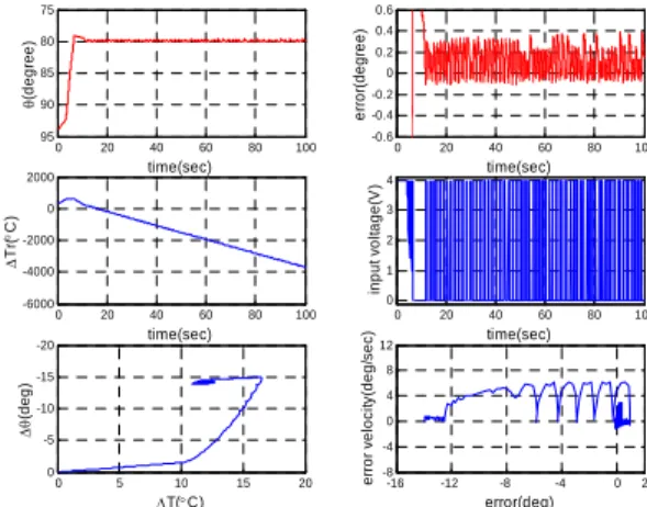
For the verifications of the above SMCTE, we conducted experiments as well as simulations with the rotary motion and bias-type SMA actuators as shown in Fig. 1. The above-mentioned SMCTE schemes were implemented by using LabVIEW® programming language by an experiment. All the control algorithms ran with a sampling frequency of 20Hz. 0 20 40 60 80 100 75 80 85 90 95 θ( degr e e) time(sec) 0 20 40 60 80 100 -0.6 -0.4 -0.2 0 0.2 0.4 0.6 er ro r( deg ree) time(sec) 0 20 40 60 80 100 -6000 -4000 -2000 0 2000 ∆ Tr (° C) time(sec) 0 20 40 60 80 100 0 1 2 3 4 input v olt ag e( V ) time(sec) 0 5 10 15 20 -20 -15 -10 -5 0 ∆θ (d e g ) ∆T(°C) -16 -12 -8 -4 0 2 -8 -4 0 4 8 12 e rro r v e lo c it y (d e g /s e c ) error(deg)
Fig. 6 Simulation result of SMCTE.
To begin with, let us see the SMCTE without boundary layer as shown in Figs 6 and 7, which show the simulation and experimental results respectively in case of a step reference command of 80 degrees. In spite of a little discrepancy between the simulation and experimental results, the overall tendency is in agreement with each other. This tells us that the derived dynamics of the SMA actuator is not only valid but the simulation is also enough to predict the experimental result.
From the time-input voltage and the error-error velocity relations, we could conclude that the SMCTE without a boundary layer has a large amplitude of the limit-cycle and a severe chattering phenomenon.
0 20 40 60 80 100 75 80 85 90 95 θ( degr e e) time(sec) 0 20 40 60 80 100 -0.6 -0.4 -0.2 0 0.2 0.4 0.6 er ro r( deg ree) time(sec) 0 20 40 60 80 100 -6000 -4000 -2000 0 2000 ∆ Tr (° C) time(sec) 0 20 40 60 80 100 0 1 2 3 4 input v olt ag e( V ) time(sec) 0 5 10 15 20 -20 -15 -10 -5 0 ∆θ (d e g ) ∆T(°C) -16 -12 -8 -4 0 2 -8 -4 0 4 8 12 e rro r v e lo c it y (d e g /s e c ) error(deg)
Fig. 7 Experimental result of the SMCTE.
From the left-bottomed figures in Fig. 6, 7, we could also find that the path lead to the minor hysteresis following the major hysteresis. From this, we can expect the steady-state will be within the major hysteresis.
0 20 40 60 80 100 75 80 85 90 95 θ( deg ree) time(sec) 0 20 40 60 80 100 -0.2 -0.1 0 0.1 0.2 e rro r(d e g re e ) time(sec) 0 20 40 60 80 100 0 400 800 1200 1600 ∆ Tr (° C) time(sec) 0 20 40 60 80 100 0 1 2 3 4 input volt age (V ) time(sec) 0 5 10 15 20 -20 -15 -10 -5 0 ∆θ (deg) ∆T(°C) -16 -12 -8 -4 0 2 -8 -4 0 4 8 12 e rr o r ve lo ci ty( d e g /se c ) error(deg)
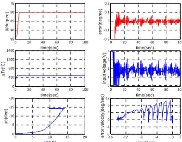
Fig. 8 Simulation result of the SMCTE with boundary layer.
0 20 40 60 80 100 75 80 85 90 95 θ( degr e e) time(sec) 0 20 40 60 80 100 -0.2 -0.1 0 0.1 0.2 er ro r( deg ree) time(sec) 0 20 40 60 80 100 0 400 800 1200 1600 ∆ Tr (° C) time(sec) 0 20 40 60 80 100 0 1 2 3 4 input v olt ag e( V ) time(sec) 0 5 10 15 20 -20 -15 -10 -5 0 ∆θ (d e g ) ∆T(°C) -16 -12 -8 -4 0 2 -8 -4 0 4 8 12 e rro r v e lo c it y (d e g /s e c ) error(deg)
Fig. 9 Experimental result of the SMCTE with boundary layer.
Now let us see the effect of the boundary layer added to the SMCTE as shown in Figs 8 and 9. The chattering phenomenon and the limit-cycle were remarkably reduced. This performance is about the same as in the TDC [10] because we used the TDC based tuning method.
Table 1 The Comparison of the applied controllers. Z.N. TDC PID SMCTE SMCTEBL RC Tsettle (sec) >100 6.1 4.8 14.4 6.2 53.7 mean error - 0.00 0.00 0.04 0.00 0.05 ∆error (deg) - 0.16 0.14 0.23 0.12 0.45 ∆errordot (deg/sec) - 2.36 2.36 3.14 2.76 4.70 -2 -1 0 1 2 -4 0 4 8 12 PID by Z.N. method er ror v e loc it y (deg/ s ec ) -2 -1 0 1 2 -4 0 4 8 12 TDC -2 -1 0 1 2 -4 0 4 8 12 PID based on TDC e rr o r ve lo ci ty( d e g /sec) -2 -1 0 1 2 -4 0 4 8 12 SMCTE -2 -1 0 1 2 -4 0 4 8 12 SMCTEBL e rro r v e lo c it y (d e g /s e c ) error(deg) -2 -1 0 1 2 -4 0 4 8 12 RC error(deg)
Fig. 10 Comparison of the limit-cycles.
Based on the four criteria, we compared 6 control schemes in Table 1: the PID control based on the Ziegler-Nichols method; the TDC; the PID control based on the TDC; the SMCTE without a boundary layer; the SMCTE with a boundary layer; the relay control. We could not reach a steady-state when a PID gain tuning is based on the Ziegler-Nichols method as shown in Fig. 10. The 3 gains of the PID control can be tuned to have the same performance as in the TDC. (See reference [12] about the detailed description.) The PID control scheme based on the TDC also shows nearly the same performance as the TDC. The relay control can be implemented by using the only discontinuous term in the bracket of Eq. (14). Among 6 controllers, the SMCTE without a boundary layer and the RC is very similar. This means that the k gain was tuned even larger than others in Eq. (14). The RC as well as the SMCTE without a boundary layer cannot have a zero error at the steady-state.
5. Conclusions
We dealt with the SMC with a time delay estimation for an application to an SMA actuator. We proposed the SMCTE with and without a boundary layer, and also studied the comparison gain tuning method based on the TDC result. The SMCTE with a boundary layer showed a good performance in terms of the various criteria. As well as the contribution of the above control methodology, the model identification for the SMA actuators was also studied. The derived dynamics
showed a continuity at the change of the phase transformation process but the original Liang’s model could not.
ACKNOWLEDGMENTS
The authors are grateful for the support provided by a grant from Atomic Energy R&D Program of Ministry of Science and Technology in Korea.
REFERENCES
[1] S. Majima, K. Kodama and T. Hasegawa, “Modeling of Shape Memory Alloy Actuator and Tracking Control System with the Model,” IEEE trans. Control Systems Technology, Vol. 9, No. 1, pp. 54-59, 2001.
[2] D. Grant and V. Hayward, “Variable Structure Control of Shape Memory Alloy Actuators,” IEEE Control Systems Magazine, Vol. 17, No. 3, pp. 80-88, 1997.
[3] A. Kumagai, P. Hozian and M. Kirkland, “Neuro-Fuzzy Based Feedback Controller for Shape Memory Alloy Actuators,” Proc. of SPIE-The International Society for Optical Engineering, 2000.
[4] D. Grant, “Accurate and rapid control of shape memory alloy actuators,” Thesis of the degree of Ph. D, McGill University, 1999.
[5] T. Hasegawa and S. Majima, “A control system to compensate the hysteresis by Preisach Model on SMA actuator,” Proc. of the 1998 9th International Symposium on Micromechatronics and Human Science, 1998. [6] T. C. Hsia and L. S. Gao, “Robot Manipulator Control
using Decentralized Time-Invariant Time-Delayed Controller,” Proc. IEEE Int. Conf. on Robotics and Automation, 1990.
[7] K. Youcef-Toumi and C. C. Shortlidge, “Control of robot Manipulator Using Time Delay,” Proc. IEEE Int. Conf. on Robotics and Automation, 1991.
[8] K. Youcef-Toumi and S. Reddy, “Dynamic Analysis and Control of High Speed and High Precision Active Magnetic Bearing,” ASME J. Dynamic Systems Measurement and Control, Vol. 114, pp. 623-632, 1992. [9] H. J. Lee and J. J. Lee, “A study on the position control
of an SMA actuator using time delay control,” Eighth international symposium on artificial life and robotics (AROB), pp. 694-697, Jan 2003.
[10] H. J. Lee and J. J. Lee, “Modeling and time delay control of shape memory alloy actuators,” Advanced Robotics, Vol. 18, No.9, pp. 881-903, 2004.
[11] J.-J. E. Slotine and W. Li, “Applied Nonlinear Control,” Prentice-Hall, 1991.
[12] H. J. Lee and J. J. Lee, “Time delay control of a shape memory alloy actuator,” Smart Materials and Structures, Vol. 13, No. 1, pp. 227-239, 2004.