1. INTRODUCTION
Time series prediction estimates the future behavior of a dynamical system based on the understanding and characterization of the system [1]. There are two basic approaches to prediction: model-based approach and model-free approach. Model-based approach assumes that sufficient prior information is available. But model-free approach does not need to know prior information. Model-free method can construct self structure only using observed current and past data. Evolvable neural networks (ENNs) are a sort of model-free approach. As a universal approximator, evolvable neural network is widely used in complex time series prediction [2]-[4].
ENNs adopt the concept of biological evolution as an adaptation mechanism [5]. ENNs with direct coding of architecture [6]-[8] use one-to-one mapping of genotype and phenotype. ENNs with direct encoding may not be practical except for small size neural networks due to high computational cost. The networks lack scalability as the size of the genetic description of a neural network grows as the network size increases [9]. Indirect encoding [10]-[14] can construct ENNs with complex network structures having repeated substructures in compact genotypes by recursive application of developmental rules. Development refers to an organization process in biological organisms, an indirect genotype-to-phenotype mapping.
This paper presents an emergent neural network model that evolves from simple structure to a network with higher connection complexity according to the developmental rules represented by the L-system [15] and the DNA coding [16]. The neural network model is a linear array of neurons. The network consists of a set of homogeneous neurons and associated connection weights with lateral connections. Neural networks are developed using the production rules of the
L-system which is represented by the DNA coding. A
chromosome in DNA coding represented an individual network. The chromosomes are mapped the set of production rules of the L-system.
Section 2 introduces the DNA coding and L-system for the development of neural networks, In Section 3, design method of ENNs is discussed. There are two steps in the design procedure: DNA encoding of L-system and the production rules for developing neural networks. The ENN developed by
the L-system are tested using prediction of chaotic time series. In Section 4, to prevent the overfitting to the given data, we propose adaptive change method of the data set for learning.
2. DEVELOPMENTAL MODEL FOR NEURAL
NETWORK EVOLUTION
2.1 DNA coding
Motivated by biological DNA, DNA coding uses four symbols A (Adenine), G (Guanine), T (Tymine), and C (Cytocine) that denote nucleotide bases, not a binary representation as in the GA. A chromosome is represented by three successive symbols called a codon. A DNA code that begins from a START codon (ATA or ATG) and ends at a STOP codon (TAA, TAG, TGA, or TGG) is translated into a meaningful code. This representation of chromosome can have multiple interpretations since the interpretations of START and STOP codons allow overlaps as shown in Fig. 1. The length of chromosomes varies. DNA coding has floating representations without fixed crossover points. Wu and Lindsay [17] proved that floating representation is effective for the representation of long chromosomes by schema analysis in GAs. The diversity of population is high since the DNA coding has a good parallel search and recombination ability. The DNA coding method can encode developmental rules without limitation of the number and the length of rule. DNA coding requires a translation table to decode codons. A codon is translated into an amino acid according to a translation table in Table 1. For example, a codon AGG is translated into an amio acid AA15. START codons ATA and
ATG are translated into AA3 within the chromosome.
CGATGCGGGAATGCCGGCCCTGACATAACT…
STARTAA6 AA8 AA2 AA7 STOP
START AA15 AA13 AA14 AA15 AA6 STOP
Gene 1
Gene 2
Fig. 1 Gene translation of a DNA sequence.
Fig. 1 shows an example of how to translate a DNA sequence. Two different translations are possible since any three symbols are grouped to a codon starting from different positions. Gene 1 is obtained from a START codon (ATG) to a STOP codon (TGA). Gene 2 appears from ATG to another
Evolvable Neural Networks for Time Series Prediction
with Adaptive Learning Interval
Dong-Wook Lee
*, Seong G. Kong
*, and Kwee-Bo Sim
***Department of Electrical and Computer Engineering, The University of Tennessee, Knoxville, TN 37919, U.S.A. (Tel : +1-865-974-3861; E-mail: {dlee27, skong}@utk.edu)
**School of Electrical and Electronic Engineering, Chung-Ang University, Seoul 156-756, Korea (Tel : +82-2-820-5319; E-mail: [email protected])
Abstract: This paper presents adaptive learning data of evolvable neural networks (ENNs) for time series prediction of nonlinear
dynamic systems. ENNs are a special class of neural networks that adopt the concept of biological evolution as a mechanism of adaptation or learning. ENNs can adapt to an environment as well as changes in the environment. ENNs used in this paper are
L-system and DNA coding based ENNs. The ENNs adopt the evolution of simultaneous network architecture and weights using
indirect encoding. In general just previous data are used for training the predictor that predicts future data. However the characteristics of data and appropriate size of learning data are usually unknown. Therefore we propose adaptive change of learning data size to predict the future data effectively. In order to verify the effectiveness of our scheme, we apply it to chaotic time series predictions of Mackey-Glass data.
STOP codon (TAA). The two genes overlap. Gene 1 results in a sequence of amio acids (protein) AA15-AA13-AA14- AA15-AA6, while Gene 2 gives AA6-AA8-AA2-AA7.
Table 1. DNA code translation table
Codon Amino acid Codon Amino acid Codon Amino acid Codon Amino acid TTT TTC AA1 TAT TAC AA9 TGT TGC AA14 TCT TCC TCA TCG AA5 TAA TAG STOP TGA TGG STOP CAT CAC AA9 CCT CCC CCA CCG AA6 CAA CAG AA10 CGT CGC CGA CGG AA15 TTA TTG CTT CTC CTA CTG ATT ATC AA2 AAT AAC AA11 AGT AGC AA16 ATA ATG AA3 / START ACT ACC ACA ACG AA7 AAA AAG AA12 AGA AGG AA15 GTT GTC GTA GTG AA4 GCT GCC GCA GCG AA8 GAT GAC GAA GAG AA13 GGT GGC GGA GGG AA17 2.2 L-system
A simple L-system can be defined as a grammar of string writing in the form G = {V, P, ω}, where V = {A1, A2, …, An}
is a finite set of alphabets Ai. P = {p1, p2, …, pn} denotes a set
of production rules pi = p(Ai). ω is an initial string
(combination of alphabets), commonly referred to as an axiom. A production rule p: V→V* maps alphabets to a set V* of finite
strings. Let Sk denote a string in the k-th rewriting step. The
rewriting procedure can be described as
) ( ) (S0 p p p S0 p S k k k 4 48 4 47 6 o L o o = = (1)
where ◦ denotes a composite operator of the rewriting operation p. The first rewriting step gives S1 = p(S0) with S0 =
ω, and S2 = p(S1) = p(p(S0)) = (p◦p)(S0) = p2(S0). For example,
consider a simple L-system with three alphabets V = {A, B, C}. Suppose the growth model G = {V, P, ω} have a set of developmental rules P = {p(A), p(B), p(C)} with p(A) = BA,
p(B) = CB, and p(C) = AC. Applying the production rules to
the axiom ω = ABC result in the strings:
BACBAC C p B p A p ABC p S p S1= ( 0)= ( )= ( ) ( ) ( )= (2) 2 ( )1 ( ) ( ) ( ) ( ) ( ) ( ) ( ) S p S p BACBAC p B p A p C p B p A p C CBBAACCBBAAC = = = = (3)
3. DESIGN OF EVOLVABLE NEURAL
NETWORKS
3.1 Structure of evolvable neural networks
The proposed evolvable neural network model consists of an array of neurons whose structure grows according to the developmental rules. A string of N symbols n1n2n3…nN,
generated from a set of production rules, finds a neural network with N nodes, ni, i = 1,2, ..., N. Fig. 2 shows the
structure of the evolvable neural network based on a developmental model. There are L input nodes and M output nodes. … i1 i2 iL o1 o2 oM … … … n1 n2 nL nL+1nL+2 nN-M-1nN-M nN-M+1 nN nN+1nN+2 nN+M
Fig. 2 Structure of the evolvable neural network with developmental models.
Nodes are connected with the connection range of the form (x, y). A pair of integers x and y (1≤ x ≤ y) configures the connection between the neighboring nodes. The parameter x denotes the index of the first node to be connected from a base node. The parameter y indicates the last node to be connected. Fig. 3 illustrates the connection of the neurons. A node at l-th location is connected to all the neurons between (l+x)-th and (l+y)-th locations. Input nodes are not connected with each other. Therefore, the indices of the first and last nodes become (l+m+x) and (l+m+y) since connection begins after skipping input neurons. … l+m+x … … l+m+1 l+m+y … l … l+m …
Fig. 3 Connection of nodes with a connection range (x, y). An evolutionary neural network is constructed from a string according to the following procedures.
1. Determine the numbers of input (L) and output (M). 2. Set the first L and the last M characters in a string to input
and output neurons. All the others are set to hidden neurons. If the total characters in a string are fewer than
L+M, then stop the construction.
3. Add M neurons as output nodes next to output neurons. 4. Connect all neurons according to connection range and the
weights.
Input and output neurons are not connceted with the neurons of the same type. Input neurons use linear activation functions while hidden and output neurons use bipolar sigmoid functions.
3.2 DNA coding for production rules
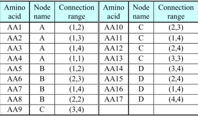
A DNA chromosome is translated into an amino acid and then into a production rule of L-system. The L-system for a mobile robot control uses four alphabets V = {A, B, C, D}. The maximum connection range is set to 4. Table 2 converts an amino acid to a node name and connection range.
Table 2. Translation table of amino acids (codons) Amino acid Node name Connection range Amino acid Node name Connection range AA1 A (1,2) AA10 C (2,3) AA2 A (1,3) AA11 C (1,4) AA3 A (1,4) AA12 C (2,4) AA4 A (1,1) AA13 C (3,3) AA5 B (1,2) AA14 D (3,4) AA6 B (2,3) AA15 D (2,4) AA7 B (1,4) AA16 D (1,4) AA8 B (2,2) AA17 D (4,4) AA9 C (3,4)
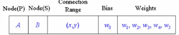
A production rule of L-system consists of alphabets, which are interpreted as nodes. The predecessor has only node but the alphabet of the successor has node name with conncetion range, bias, and weights. Fig. 5 shows a production rule of the form p(A) = B with connection range (x,y). A production rule is composed of nine codons corresponding a predecessor node, a successor node, a connection range, a bias, five connection weights. Five weights are needed since the maximum connection range is set to 5. A single predecessor node can have multiple sucessor nodes as in the rule p(A) = BC.
Fig. 4 DNA coding of a production rule.
Bias and weights are real values calculated by Eq. (4). The bias and weights have values of bound from -3.2 to 3.1 at 0.1 intervals.
(
2 1 0)
2 4 1 4 0 4 32 10 b b b w= ⋅ + ⋅ + ⋅ − (4)where b0, b1, and b2 are the three DNA symbols of the codon
(e.g. ACG). The values of each DNA symbol are T = 0, C = 1,
A = 2, and G = 3.
Fig. 5 shows an example of translating a DNA code into a production rule. Two production rules can be created since two START codons (ATG) exist in the chromosome. The codon TAC followed by ATG is translated to AA9 (Node C) according toTable 2. The next codon CGG is translated to AA15 (Node D). The next codon (CGT) is also translated to AA15, which corresponds to the connection range (2,4). The following codon (GAA) denotes a bias of the value 2.6 (=[3×42+2×41+2×40-32]/10). The next five codons determine
weight values. This procedure is repeated for the next production rule until the STOP codon is met. The first rule is represented by p(C) = D(2,4)A(4,4). The second rule p(B) =
D(3,4) is obtained from the different reading frame. Not-used
codons are denoted by ‘NU.’ If multiple rules have the same predecessor but different successors as in p(A) = B and p(A) =
CB, only the first rule p(A) = B is used, and the others are
eliminated. If no rule is found for a predecessor Ai, a rule p(Ai)
= Ai is used.
CGATGTACCGGCGTGAATGCCGGGGTGCACGGCTCGGGACAACCACCGTTAGCGTTGATTAACG ….
STARTAA6 AA17 AA14 NU NU NUSTOP
START AA9 AA15 AA15 AA2 AA17 NU STOP
Rule 1
Rule 2
D (3,4) 0.7 2.0 -0.1 2.5 0.9 -0.7 B
(AA17) (AA14) ACG GCT CGG GAC AAC CAC
(AA6) Rule 2
A (4,4) 0.6 0.5 0.5 1.6 1.3 1.6 D (2,4) 2.6 -1.9 -0.1 2.8 -1.0 -0.1
C
(AA2) (AA17) ACA ACC ACC GTT AGC GTT (AA15) (AA15) GAA TGC CGG GGT CCA CGG
(AA9)
Rule 1
successor predecessor
Fig. 5 Interpretation of production rules from a DNA code.
4. TIME SERIES PREDICTION EXPERIMENT
4.1 Time series predictionGenerally, the problem of time series prediction is to find a function that predicts a future value x(t+I) from the current and the past values (x(t), x(t-D), …, x(t-qD)) where t is time index, I (I > 0) is the time step to be predicted, q is the order of
the model or the embedding dimension, and D (D ≥ 1) is time delay. Then the time series prediction is represented by a form of function: ) ( , ), 2 ( ), ( ), ( ( ) ( ˆ t I F xt xt D xt D xt qD x + = − − L − (5)
To validate our method, we use well investigated time series data, namely Mackey-Glass chaotic data. The equation of Mackey-Glass time series is as follows [18].
) ( ) ( 1 ) ( ) ( t bx t x t ax dt t dx c − − + − = τ τ (6)
where the variables are chosen to be a = 0.2, b = 0.1, c = 10 and τ equal to 30 in this paper. The data is generated by fourth order Runge-Kutta method of (6).
The inputs to the proposed ENN are the time series in lagged space x(t), x(t-D), x(t-2D), and x(t-3D). The output is the predictive value of x(t+I), with I = D = 5. So minimum 4 input neurons and 1 output neuron are needed for evaluating an ENN. Therefore the ENN that has less than 5 neurons is not evaluated and the fitness becomes 0.
Generally, as the error decreases, the fitness must increase. So we use the fitness function for ENN as
) (t
E
e
Fitness= −λ⋅ (7)
where λ is the parameter that determines the slope of the curves, E(t) is normalized mean square error (NMSE) at time t. In experiment, λ is set as 5 because NMSE is less than 0.5 in most cases.
The performance of the evolutionary neural network is evaluated by estimating the NMSE which is defined as
∑
∑
∑
− = − = − = ⎟⎟ ⎠ ⎞ ⎜⎜ ⎝ ⎛ − − − − − − = 1 0 2 1 0 1 0 2 ) ( 1 ) ( )) ( ˆ ) ( ( ) ( N k N i N k i t x N k t x k t x k t x t E (8)where N is the number of previous data to be tested in current evaluation, x(t) is the ideal or observed time series, xˆ t() is the predicted times series. Because the NMSE include the variance of the data, we can compare the performance of our model with the performance of previous works regardless of the training set size.
4.2 Adaptive learning interval
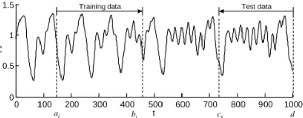
To prevent ENN from overfitting to the given data, we propose adaptive change method of the data set for evaluation. In general optimal size of training data is not given and is hard to predict. But it is very important factor to obtain a good performance. So in this paper adaptive increment method of training data is presented. The problem of time series prediction is to predict next unknown data using given data. However using all data for training cause very slow learning and sometimes impossible to continue training. So we start to train using small sized data and increase the data size gradually by introducing test data. Test data is used to determine whether the training data increase or not. So we pick up test data from the back of known data set. It is shown at Fig. 6.
Brief algorithm is as follows. In each generation, the data set used is Pi samples for training and Qi samples for testing
where i is the index of data, Pi and Qi is positive variable. All
individuals in each generation are evaluated using same training data. After the evaluation of all individuals, the best individual is evaluated using test data. If the performance to
the test data is worse than that to the training data then we increase the training data in the next generation. In this case we use decision function as (9) to decide whether we generate new data or not.
train
test E
E >(1+δ)⋅ (9) where Etest and Etrain are the NMSE of the best individual to
the test and the training data. δ is a positive parameter that represents a tolerance. 0 100 200 300 400 500 600 700 800 900 1000 0 0.5 1 1.5 t x( t)
Training data Test data
bi
ai ci d
Fig. 6 Adaptive increment of data set for evolving neural networks.
We introduce acceptable maximum size of training data,
Pmax. If the size of training data reaches Pmax then the size of
training data does not increase and only change the range that covered. Algorithm 1 shows the detailed explanation for adapting the data size.
Algorithm 1: Adaptive Learning Interval Algorithm
In Algorithm 1, Etest,i and Etrain,i are the NMSE of the best
individual of current generation to the test and the training data, Eobj is the objective performance, Pi and Qi is the size of
training and test data in ith index, ∆ is the increasing or decreasing data size, δ is a positive parameter that represents a tolerance, and δ ≥ 1, T is the size of known data.
Fig. 6 shows the adaptive increment of training and test data by Algorithm 1. In case that Etest is worse than (1+δ)⋅Etrain,
training data are insufficient to cover the test data. Therefore we increase the size of training data. In case that Etest is better
than (1+δ)⋅Etrain, we maintain the training data and increase
the size of test data. In earlier phase, we can expect that the size of both training and test data will increase. In latter phase, after sufficient training data are obtained, only the size of test data will increase. As the training data increase, calculation cost also increases. However, the increase of test data does not increase the calculation cost because all individuals are evaluated by training data and only the best one are evaluated by both training and test data.
To evaluate the effectiveness of Algorithm 1, we compare the results using Algorithm 1 and without Algorithm 1. By experiment, the MMSE of evolved neural network without Algorithm 1 was 2.70×10⁻³ and the MMSE of evolved neural
network with Algorithm 1 was 2.35×10⁻³. The performance of
prediction is improved by using Algorithm 1.
Evolved L-system is G = {V, P, ω} with V = {A, B, C, D}, and ω = A, where the generated rules by DNA code are each
p1: p(A) = AAAB, p2: p(B) = BC, p3: p(C) = C, and p4: p(D) =
BA. Growth sequence of neural network is follows. The rule p4
is not used in this case because the successor of from p1 to p3
does not have symbol D. S1: AAAB
S
2: AAABAAABAAABBC (10)
S3: AAABAAABAAABBCAAABAAABAAABBCAAAB AAABAAABBCBCC
Fig. 7 shows the architecture of evolved neural network, which is visualization of S3. Input to the ENN is the values of
time series (x(t), x(t-5), x(t-10), x(t-15)) and the output is ) 5 ( ˆt+ x . … x(t) x(t-5) x(t-15) n1 n2 n4 n5 n6 n8 n9 n45 n3 x(t-10) n7 n10 n11 n39 n40 n41 n42 n43 n44 ) 5 ( ˆt+ x
Fig. 7 Evolved neural network architecture for Mackey-Glass time series prediction.
5. CONCLUSION
In this paper, we proposed a new method of constructing neural networks and an adaptive learning interval algorithm in time series prediction. Proposed neural networks are based on the concept of development and evolution. To make evolvable neural networks, we utilize DNA coding method, L-system and evolutionary algorithm. Evolutionary neural networks are constructed from the string that is generated by production rules of L-system. DNA coding has no limitation in expressing the production rules of L-system. Therefore evolutionary neural network are effectively designed by L-system and DNA coding method. Proposed ENN is applied to time series prediction problem. By adaptive learning interval algorithm, the performance of prediction is improved.
ACKNOWLEDGMENTS
This research was supported by the Brain Neuroinformatics Research Program by Ministry of Commerce, Industry and Energy
1. Index i ← 0, and set the parameters P0 (a = 0, b0 = P0
- 1), Q0 (c0 = T - Q0, d = T - 1), Pmax, and δ, Eobj,
where P0 + Q0 << T, T is number of given data. In
this case, P0 and Q0 are set as acceptable minimal
number of data by designer, Pmax is set as acceptable
maximum number of training data, and Eobj is
objective MMSE value for termination.
2. Perform evolutionary algorithm for G ≥ 1 genera- tions. After G generations, calculate Etrain,i and Etest,i.
3. If Etrain,i ≤ Eobj, Etest,i ≤ Eobj then go to step 6.
4. (1) If Etest,i > (1+δ)⋅Etrain,i then increase the training
data size and maintain the test data size, i.e. Pi+1 = Pi
+ ∆, Qi+1 = Qi.
In this case, b i+1 = bi + ∆, ci+1 = ci. But after the
renewal of bi and ci, if ci+1 ≤ bi+1 ≤ c0 then ci+1 = bi+1
else if bi+1 > c0 then bi+1 = ci+1 = c0.
If Pi+1 > Pmax then ai+1 = bi+1 - Pmax else ai+1 = ai.
(2) If Etest,i≤ (1+δ)⋅ Etrain,i then maintain the training
data size and increase the test data size, i.e. Pi+1 = Pi,
Qi+1 = Qi + ∆.
In this case ai+1 = ai, bi+1 = bi, ci+1 = ci - ∆. But after
the renewal of bi and ci, if ci+1 < bi+1 then ci+1 = bi+1.
5. i = i + 1 and return to step 2.
6. Stop the evolution and get the best individual as
REFERENCES
[1] M. S. Kim and S. G. Kong, “Parallel-structure fuzzy system for time series prediction,” Int. J. of Fuzzy
Systems, Vol. 3, No. 1, pp.331-339, 2001.
[2] J. R. McDonnell and D. Waagen, “Evolving Recurrent Perceptrons for time-series modeling,” IEEE Trans. on
Neural Networks, Vol 5, No. 1, pp.24-38, 1994.
[3] H. A. Mayer and R. Schwaiger, “Evolutionary and coevolutionary approaches to time series prediction using generalized multi-layer predictions,” Proc. of
Congress on Evolutionary Computation, Vol. 1,
pp.275-280, 1999.
[4] S. G. Kong, “Time series prediction with evolvable block-based neural networks,” Proc. of Int. Joint Conf.
on Neural Networks (IJCNN), 2004.
[5] X. Yao, “Evolving artificial neural networks,”
Proceedings of the IEEE, Vol. 87, No. 9, pp.1423-1447,
1999.
[6] S. W. Moon and S. G. Kong, “Block-based Neural Networks,” IEEE Trans. on Neural Networks, Vol. 12, No. 2, pp.307-317, 2001.
[7] P. J. Angeline, G. M. Sauders, and J. B. Pollack, “An evolutionary algorithm that constructs recurrent neural networks,” IEEE Trans. on Neural Networks, Vol. 5, No. 1, pp.54-65, 1994.
[8] X. Yao and Y. Lie, “A new evolutionary system for evolving artificial neural networks,” IEEE Trans. on
Neural Networks, Vol. 8, No. 3, pp.54-65, 1994.
[9] F. H. F. Leung, H. K. Lam, S. H. Ling, and P. K. S. Tam, “Tuning of the structure and parameters of neural network using an improved genetic algorithm,” IEEE
Trans. on Neural Networks, Vol. 14, No. 1, pp.79-88,
2003.
[10] J. Kodjabachian and J. A. Meyer, “Evolution and development of neural controllers for locomotion, gradient-following, and obstacle-avoidance in artificial insects,” IEEE Trans. on Neural Networks, Vol. 9, No. 5, pp.796-812, 1998.
[11] B. L. M Happel and J. M. J. Murre, “The design and evolution of modular neural network architecture,”
Neural Networks, Vol. 7, pp.985-1004, 1994.
[12] E. J. W. Boers and I. G. Sprinkhuizen-Kuyper, “Combined biological metaphors,” Advances in the
Evolutionary Synthesis of Intelligent Agents, M. J. Patel,
V. Honavar, and K. Balakrishnan, Eds., MIT Press, Ch. 6, pp.153-183, 2001.
[13] F. Gruau, “Automatic definition of modular neural networks,” Adaptive Behavior, Vol. 3, No. 2, pp.151-183, 1995.
[14] A. Cangelosi, S. Nolfi, and D. Parisi, “Artificial life models of neural development,” On Growth, Form and
Computers, S. Kumar and P. J. Bently, Eds., Elsevier
Academic Press, pp.339-352, 2003.
[15] A. Lindenmayer, “Mathematical models for cellular interaction in development, Part I, II,” Journal of
Theoretical Biology, Vol. 18, No. 3, pp.280-315, 1968.
[16] Y. Yoshikawa, T. Furuhashi, and Y. Uchikawa, “Knowledge acquisition of fuzzy control rules using DNA coding method and pseudo-bacterial GA,” Lecture
Notes in Artificial Intelligence, Springer, Vol. 1285,
pp.126-135, 1997.
[17] A. S. Wu and R. K. Lindsay, “A computation of the fixed and floating building block representation in genetic algorithms,” Evolutionary Computation, Vol. 4, No. 2, pp.169-193, 1996.
[18] M. C. Mackey and L. Glass, “Oscillation and chaos in physiological control systems,” Science, Vol. 197, pp.287-289, 1977.