Development of the Multi-dimensional Fluid Dynamics Code and
Benchmarking for the Natural Circulation Problem
B.U. Baea*, H.Y. Yoonb, B.G. Huhc, D.J. Euhb, B.J. Yunb, C.H. Songb, G.C. Parka
a Department of Nuclear Engineering, Seoul National Unviersity, Seoul,151-742, Korea, b Korea Atomic Energy Research Institute, P.O. Box 105, Yuseong, Daejeon, 305-600, Korea
c Korea Institute of Nuclear Safety, P.O. Box 19, Yuseong, Daejeon, 305-600, Korea * E-mail : [email protected]
1. Introduction
In the analysis of two-fluid model, the interfacial area concentration (IAC) is one of the most important parameters with respect to the interfacial transfer terms between two phases. Recently, instead of the conventional static approach for modeling IAC, the IAC transport equation was developed for adiabatic bubbly flow or nucleate boiling flow[1].
This study is a part of the development of computational fluid dynamics code for analyzing the boiling flow with two-fluid model and IAC transport equation. Multi-dimensional approach was utilized in order to overcome the limitation in one-dimensional modeling for the IAC transport equation. The problem for single-phase natural circulation was used for benchmarking of the code as a first step for checking the robustness of the developed code
2. Development of the Fluid Dynamics Code
2.1 Governing equation
The governing equations for the two-phase flow analysis that are used in this study are as follows:[2]
(
k k)
(
)
k k kv k t α ρ α ρ ∂ + ∇ ⋅ = Γ ∂ (1) ( k k k) ( ) ( )(
T)
k k k k k k k k k k k ki k ik k ki ki k v v v p t g v M p α ρ α ρ α α τ τ α ρ α τ α ∂ ⎡ ⎤ + ∇ ⋅ = −∇ + ∇ ⋅⎢ + ⎥ ⎣ ⎦ ∂ + + Γ + − ∇ ⋅ + ∇ (2)(
)
(
)
(
)
" k k k T k k k k k k k k k k ki k i k k H H v q q t D p H a q Dt α ρ α ρ α α φ ∂ ⎡ ⎤ + ∇ ⋅ = −∇ ⋅⎢ + ⎥ ⎣ ⎦ ∂ + + Γ + + (3) In discretizing the above equations, the finite volume method (FVM) was used with non-staggerd grid for the numerical stability. That is, each term in the equation was integrated over the cell volume and then defined at the center of cell.2.2 Numerical scheme
For the advancement of the time, the explicit Euler method was used in the code. The momentum equation for each phase is solved so that the superficial velocity
(φk=αk kv ) and the pressure at next time step are
calculated. For solving the matrix of pressure correction,
the Simplified Marker and Cell (SMAC) algorithm was
adopted with considering the term for phase change,
Γ
k.And then enthalpy at the next time step is estimated in the energy equation.
2.3 Closure relations
In the momentum equation, the closure relations are necessary in terms of the interfacial momentum transfer,
ik
M , including the drag, virtual mass force and lift
force. The correlations for these are listed in the literature.[3]
For the dynamic modeling, the IAC transport equation should be implemented in the future. In this work, as a preliminary test for overall robustness of the code, the conventional correlation of Anglart et al. was utilized for IAC[4].
3. Benchmark for Natural Circulation
3.1 Definition of the problem
The problem proposed by De Vahl Davis[5] is about the natural circulation of single phase in a square as shown in Figure 1. The temperatures at left and right
side are maintained as TH and TC, respectively, and the
upper and lower side are insulated.
Figure 1. Geometry for benchmark problem
The test condition is given with respect to Rayleigh number defined as;
(
)
2 3 2 Pr H C g T T L Ra ρ β µ − = (4)The standard solutions are known for the cases of
Ra=103, 104, 105, and 106. In the application of this
study, the working fluid was water at the atmospheric
pressure and TH and TC was fixed as 80℃ and 30℃,
respectively. Therefore, the size of square, L, was
Transactions of the Korean Nuclear Society Autumn Meeting Busan, Korea, October 27-28, 2005
determined so as to satisfy the Rayleigh number of the above value. Then the grid was generated with the structured 40X40 cells. The test geometry for four cases are summarized in Table 1.
Table 1. Test conditions
Ra L(m) Cell size (=L/40,m)
103 9.910 × 10⁻⁴ 2.478 × 10⁻⁵
104 2.135 × 10⁻³ 5.338 × 10⁻⁵
105 4.600 × 10⁻³ 1.150 × 10⁻⁴
106 9.910 × 10⁻³ 2.478 × 10⁻⁴
3.2 Results of temperature and velocity
The results of the temperature and velocity profile for
the cases of Ra=103 and 106 are presented in the Figures
2, 3, 4 and 5. As shown in the results, the developed code reasonably simulates the two-dimensional behavior of natural circulation.
X Y 0 0.0005 0.001 0 0.0001 0.0002 0.0003 0.0004 0.0005 0.0006 0.0007 0.0008 0.0009 0.001 Tf 80 77.5 75 72.5 70 67.5 65 62.5 60 57.5 55 52.5 50 47.5 45 42.5 40 37.5 35 32.5 30 Frame 001⏐ 05 Sep 2005 ⏐ 9.99990999999003 Frame 001⏐ 05 Sep 2005 ⏐ 9.99990999999003
Figure 2. Temperature distribution (Ra=103)
X Y 0 0.005 0.01 0 0.001 0.002 0.003 0.004 0.005 0.006 0.007 0.008 0.009 0.01 Tf 80 77.5 75 72.5 70 67.5 65 62.5 60 57.5 55 52.5 50 47.5 45 42.5 40 37.5 35 32.5 30 Frame 001⏐ 05 Sep 2005 ⏐ 150.000010000352 Frame 001⏐ 05 Sep 2005 ⏐ 150.000010000352
Figure 3. Temperature distribution (Ra=106)
X Y 0 0.0005 0.001 0 0.0001 0.0002 0.0003 0.0004 0.0005 0.0006 0.0007 0.0008 0.0009 0.001 0.001m/s Frame 001⏐ 05 Sep 2005 ⏐ 9.99990999999003 Frame 001⏐ 05 Sep 2005 ⏐ 9.99990999999003
Figure 4. Velocity field (Ra=103)
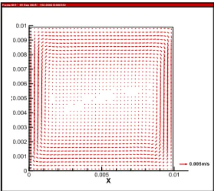
X Y 0 0.005 0.01 0 0.001 0.002 0.003 0.004 0.005 0.006 0.007 0.008 0.009 0.01 0.005m/s Frame 001⏐ 05 Sep 2005 ⏐ 150.000010000352 Frame 001⏐ 05 Sep 2005 ⏐ 150.000010000352
Figure 5. Velocity field (Ra=106) 3.3 Comparison of Nusselt number
From the temperature gradient near the wall, the average Nusselt number can be obtained as follows.
0 1 L 1 y i H C w L T Nu Nu dy y L L T T x ∂ ⎛ ⎞ = = ⎜ ⎟ ∆ − ⎝∂ ⎠
∑
∫
(5)The Nusselt numbers in this study and the literature were compared in Table 2. It shows the reasonable agreement between the developed code and the standard solution.
Table 2. Comparison of Nusselt number
Ra (Hot / Cold plate) CFD (De Vahl Daivs, 1983)Reference
103 1.130 / 1.130 1.118
104 2.310 / 2.310 2.243
105 4.903 / 4.903 4.519
106 10.13 / 10.12 8.8
4. Conclusion
In order to realistically analyze the two-phase flow, multi-dimensional fluid dynamics code was developed with the two-fluid model and FVM. Also, by comparing with the benchmark problem for the natural circulation, the preliminary estimation for the overall robustness of the code was evaluated.
In the future, the IAC transport equation will be implemented into the code to dynamically model the interfacial transfer terms. Then the code is expected to reasonably simulate the multi-dimensional boiling flow.
REFERENCES
[1] S. J. Kim, Research on interfacial area transport : The present and future efforts, NURETH-10, Seoul, Korea, 2003 [2] M. Ishii and et al., Two-fluid model and hydrodynamic constitutive relations, Nuclear Engineering and Design, vol. 82, pp. 107-126, 1984
[3] B. G. Huh, Experimental and analytical study of interfacial area transport in a vertical two-phase flow, Ph. D. Thesis, Seoul National University, 2005
[4] H. Anglart et al., CFD prediction of flow and phase distribution in fuel assemblies with spacers, Nuclear Engineering and Design,vol. 177, pp. 215-228, 1997
[5] G. de Vahl Davis, Natural convection of air in a square cavity: a benchmark numerical solution, Int. J. Number. Methods Fluids 3, pp. 249-264, 1983