Journal of Magnetics 22(2), 257-265 (2017) https://doi.org/10.4283/JMAG.2017.22.2.257
©2017 Journal of Magnetics
Analysis and Optimization of the Axial Flux Permanent Magnet
Synchronous Generator using an Analytical Method
Junaid Ikram1, Nasrullah Khan1, Qudsia Junaid2, Salman Khaliq3, and Byung-il Kwon4* 1COMSATS Institute of Information Technology, Islamabad, Pakistan
2National Transmission and Dispatch Company, Islamabad, Pakistan 3Intelligent Mechatronics Research Center, KETI, Korea
4Hanyang University, Ansan, Korea
(Received 26 January 2017, Received in final form 15 May 2017, Accepted 18 May 2017)
This paper presents a 2-D analytical method to calculate the back EMF of the axial flux permanent magnet synchronous generator (AFPMSG) with coreless stator and dual rotor having magnets mounted on both sides of rotor yoke. Furthermore, in order to reduce the no load voltage total harmonics distortion (VTHD), the ini-tial model of the coreless AFPMSG is optimized by using a developed analytical method. Optimization using the 2-D analytical method reduces the optimization time to less than a minute. The back EMF obtained by using the 2-D analytical method is verified by a time stepped 3-D finite element analysis (FEA) for both the ini-tial and optimized model. Finally, the VTHD, output torque and torque ripples of both the iniini-tial and opti-mized models are compared with 3D-FEA. The result shows that the optiopti-mized model reduces the VTHD and torque ripples as compared to the initial model. Furthermore, the result also shows that output torque increases as the result of the optimization.
Keywords : axial flux permanent magnet synchronous generator, 2-D analytical method, no load voltage total har-monics distortion, Finite element analysis
1. Introduction
The axial flux Permanent magnet synchronous gene-rator (AFPMSG) is suitable for low speed wind power generation due to its higher torque density [1, 2]. It has the advantages of a larger power to weight ratio and better cooling than radial flux topologies [3, 4]. Further-more, the coreless stator topology of the AFPMSG reduces the generator weight and it has a lower cogging torque and unbalanced axial force [5, 6]. The coreless AFPMSG also has the advantage of high efficiency [7].
The computation of the air gap magnetic field di-stribution is important because it is required for the calculation of back EMF and torque. The computation of the magnetic field in an AFPMSG is done by using the magnetic equivalent circuit method, an analytical method for solving Maxwell’s equations, or the finite element analysis (FEA). Although the FEA is more accurate
com-pared to the analytical method, due to the nonlinear fields in electrical machines, the effect of individual generator dimensions on the field distribution may not be easily identified and the method is very time consuming [8, 9]. Therefore, analytical methods are favored for finding a time-efficient solution.
The magnetic flux distribution in a PM machine is computed either by using a polar or rectangular coordi-nate system [10, 11]. Magnetic field computation of axial flux PM machines have been a focus of research in recent years. The field calculations of the double sided axial flux machine with slot-less stator are computed by represent-ing magnets and coils as current sheets in [12]. An analy-tical method of the normal field component was develop-ed for the single stator and rotor axial flux machine with flat multiple pole disc magnets by using the mean radius approach [13]. The magnetic field distribution of a single sided axial flux PM generator with a coreless stator has also been computed using the mean radius approach [14]. A voltage total harmonic distortion (VTHD) calculation of the single-sided coreless AFPMSG using a 2-D analy-tical method is presented in [14]. The optimization for the
©The Korean Magnetics Society. All rights reserved. *Corresponding author: Tel: +82-31-400-5165 Fax: +82-31-409-1277, e-mail: [email protected]
reduction in VTHD of the double sided AFPMSG using 3-D FEA is presented in [15]. However, an analytical solution of the magnetic field distribution of a coreless dual rotor single stator AFPMSG has not been presented yet, which uses the mean radius approach.
This paper presents a 2-D analytical method to optimize an AFPMSG having coreless stator and dual rotor yokes with PMs mounted on them. The developed analytical method is an extension of the analytical method developed in [14]. The analytical method presented in [14] is for coreless stator and sector shaped PMs are mounted on the inner side of one rotor yoke. Whereas, the developed analytical method presented in this paper is for coreless stator and sector shaped PMs are mounted on the inner side of both the rotor yokes. The equations are developed by using the same approach i.e. mean radius, rectangular coordinate system and solution of the Maxwell's equations as was presented in [14]. However, there is a minor difference in the derived equations and the equations that were presented in reference [14] due to the different position of lower and upper magnets from the reference point. In the developed analytical method equations are not being simply taken from the references [12-14] for the superposition but they are derived. Furthermore, developed analytical method is used for the optimization of the AFPMSG with coreless stator and PMs mounted on both sides of the rotor yokes. Optimization using the analytical method is done in order to reduce the time. Genetic algorithm and direct search method are employed on the developed analytical method for an optimal design of the AFPMSG. A transient 3-D FEA is used to verify the results of the developed 2-D analytical method for both the initial and optimized models. JMAG designer ver. 14.1 is used as a 3D-FEA tool in this paper. Performance comparison of AFPMSG's initial and optimized models under no load and load conditions is done with time stepping FEA. Due to dynamic behavior of the electric machines time stepping FEA is more accurate as compared to the magneto-static FEA. Furthermore time stepping FEA gives the results directly without recourse to further assumptions and calculations [16]. Finally, the VTHD, output torque and torque ripple of the initial and optimized models are compared using 3-D FEA.
The rest of this article is arranged as follows: Section II presents the 2-D analytical method for the modeling and analysis of coreless AFPMSGs. This is followed by Section III, which describes the optimization of the AFPMSG using the developed analytical method. In Section IV, a conclusion is drawn.
2. A 2-D Analytical Method for the
Modeling and Analysis of Coreless
AFPMSG
This section presents the 2-D analytical method for calculating the magnetic field density with Maxwell’s equations using boundary conditions of the single coreless stator and dual rotor AFPMSG.
2.1. Initial Model
Figure 1 shows the initial model of the 1.0 kW, three phase, Y-connected, double-sided AFPMSG. The AFPMSG has two disc-shaped rotor yokes with permanent magnets placed on it. The coreless stator is sandwiched between two rotors and has stator windings fixed by the plastic resin. Three phases of the stator windings are arrayed periodically in the circumferential direction. Table 1 shows the design parameters of the AFPMSG for the 2-D
Fig. 1. (Color online) Exploded view of the 3-D FEA model of the AFPMSG.
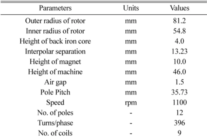
Table 1. Parameters of the AFPMSG model.
Parameters Units Values
Outer radius of rotor mm 81.2 Inner radius of rotor mm 54.8 Height of back iron core mm 4.0
Interpolar separation mm 13.23 Height of magnet mm 10.0 Height of machine mm 46.0 Air gap mm 1.5 Pole Pitch mm 35.73 Speed rpm 1100 No. of poles - 12 Turns/phase - 396 No. of coils - 9
analytical method.
2.2. 2-D Analytical Method
For computation of the magnetic field, the mean radius approach and the rectangular coordinate system that is presented in [12-14] is used. Therefore, the 3-D geometry of the AFPMSG is converted into a 2-D linear model in which the X-axis represents the circumferential direction and the Y-axis represents the axial direction. The compu-tation of the no load magnetic flux density components by the 2-D analytical method in the air gap and magnet regions is based on the solution of Maxwell's equations using the boundary condition method. In order to obtain the analytical solution and simplify the derivation of the analytical method, the following assumptions are made: There is no magnetic saturation and the rotor back iron has infinite permeability, the permanent magnets have uniform magnetization and have constant relative recoil permeability, and eddy currents are negligible.
To calculate the magnetic field by the individual rotor, one side's permanent magnets were neglected when cal-culating the magnetic flux density due to the other side's magnets. Furthermore, the coil region permeability is con-sidered the same as the air gap region in the calculation of magnetic field due to upper and lower rotors magnets. The net magnetic field in the machine is the summation of magnetic fields due to both rotor permanent magnets. Figure 2 shows the AFPMSG linear model for the computation of the no load magnetic field due to the lower rotor permanent magnets. For permanent magnet machines with linear demagnetization characteristics, the Laplacian equation governs the scalar magnetic potential in both the air gap and permanent magnet regions [14]. The general solutions of the Laplacian equation in the air gap and magnet regions are given by Equations (1) and (2), respectively.
(1)
(2)
Where φ is the magnetic scalar potential with subscripts represents regions, y is the axial height, τp is pole pitch, n is harmonic order and x is the circumferential distance.
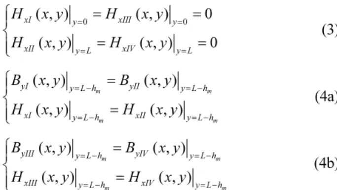
The coefficients D1 to D4 in the above expressions are determined by imposing the boundary conditions. The magnetic field due to permanent magnets must satisfy the boundary conditions given in Equation (3) and (4) [11].
(3)
(4a)
(4b)
Where Hx is the circumferential components of the magnetic field intensity and By is the axial component of the magnetic flux density.
By employing the above mentioned boundary conditions, we get the values of the coefficients given by Equations (5-8). (5) (6) (7) (8) Here, and,
Where hm is axial length of the magnet, αp is the pole arc to pole pitch ratio, L is the axial height of the machine, Br is the residual flux density of the PM, μo is the
perme-1 2 1,3,5,... ( )cos( ) ∞ − = = =
∑
n yp + n yp p I III n n x D eτπ D e τπ π ϕ ϕ τ 3 4 1,3,5,... ( )cos( ) ∞ − = = =∑
n yp + n yp p II IV n n x D eτπ D e τπ π ϕ ϕ τ 0 0 ( , ) ( , ) 0 ( , ) ( , ) 0 = = = = ⎧ = = ⎪ ⎨ = = ⎪⎩ xI y xIII y xII y L xIV y L H x y H x y H x y H x y ( , ) ( , ) ( , ) ( , ) = − = − = − = − ⎧ = ⎪ ⎨ = ⎪⎩ m m m m yI y L h yII y L h xI y L h xII y L h B x y B x y H x y H x y ( , ) ( , ) ( , ) ( , ) = − = − = − = − ⎧ = ⎪ ⎨ = ⎪⎩ m m m m yIII y L h yIV y L h xIII y L h xIV y L h B x y B x y H x y H x y 1 sinh ( ) 2 = − Δ n p m p M n h D n τ π τ π 2 sinh( ) 2 = Δ n p m p M n h D n τ π τ π 3 sinh ( ( ) ) 2 − = Δ p n p m p n L M n L h D n eπ τ τ π τ π 4 sinh ( ( ) ) 2 − − = − Δ p n p m p n L M n L h D n e π τ τ π τ π ( ) cosh sinh ( ) cosh sinh − ⎛ ⎞ ⎛ ⎞ Δ = ⎜ ⎟ ⎜ ⎟ ⎝ ⎠ ⎝ ⎠ − ⎛ ⎞ ⎛ ⎞ + ⎜ ⎟ ⎜ ⎟ ⎝ ⎠ ⎝ ⎠ p p m m r p m m p p n h n L h n L h n h π π τ μ τ τ π π τ τ 0 sin( 2) 2 2 = r p n p p n B M n π α α μ π αFig. 2. (Color online) Linear representation of the AFPMSG for the lower rotor.
ability of the free space and µr is the recoil permeability of the PM.
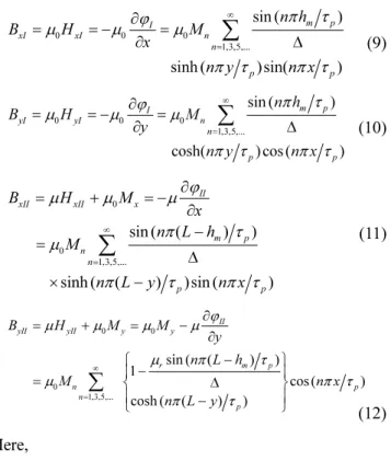
By substituting the above computed coefficients into Equations (1) and (2) and by solving for the magnetic field, we get the circumferential and axial components of the magnetic field. The magnetic field components due to the lower magnets in the air gap and magnet regions are given by Equations (9-12). (9) (10) (11) (12) Here, µ = µ0µr
Where Bx is the circumferential component of the flux density, By is the axial component of the flux density, Hx is the circumferential component of the field intensity and Hy is the axial component of the field intensity.
Figure 3 shows the linear model of the AFPMSG for
the computation of the no load magnetic field due to the upper rotor magnets. The circumferential and axial components of magnetic flux density due to upper rotor magnets in the air gap and magnet regions are given by Equations (13-16).
(13)
(14)
(15)
(16)
The armature reaction refers to the magnetic field produced by currents in the stator coils and their inter-action with the field flux. The disc armature winding is considered as thin current sheets. Figure 4 shows the linear model of the AFPMSG for the computation of the armature reaction field. The axial component of the armature reaction is given by Equation (17) [3].
(17) 0 0 0 1,3,5,... sin ( ) sinh ( )sin( ) ∞ = ∂ = = − = ∂
∑
Δ m p I xI xI n n p p n h B H M x n y n x π τ ϕ μ μ μ π τ π τ 0 0 0 1,3,5,... sin ( ) cosh( )cos( ) ∞ = ∂ = = − = ∂∑
Δ m p I yI yI n n p p n h B H M y n y n x π τ ϕ μ μ μ π τ π τ 0 0 1,3,5,... sin ( ( ) ) sinh ( ( ) )sin ( ) ∞ = ∂ = + = − ∂ − = Δ × −∑
II xII xII x m p n n p p B H M x n L h M n L y n x ϕ μ μ μ π τ μ π τ π τ 0 0 0 1,3,5,... sin ( ( ) ) 1 cos( ) cosh ( ( ) ) ∞ = ∂ = + = − ∂ − ⎧ − ⎫ ⎪ ⎪ = ⎨ Δ ⎬ ⎪ − ⎪ ⎩ ⎭∑
II yII yII y y r m p n p n p B H M M y n L h M n x n L y ϕ μ μ μ μ μ π τ μ π τ π τ 0 0 0 1,3,5,... sin ( ) sinh ( ( ) )sin ( ) ∞ = ∂ = = − = ∂ Δ × −∑
m p III xIII xIII n n p p n h B H M x n L y n x π τ ϕ μ μ μ π τ π τ 0 0 0 1,3,5,... sin ( ) cosh ( ( ) )cos( ) ∞ = ∂ = = − = ∂ Δ × −∑
m p III yIII yIII n n p p n h B H M y n L y n x π τ ϕ μ μ μ π τ π τ 0 0 1,3,5,... sin ( ( ) ) sinh ( )sin( ) ∞ = ∂ = + = − ∂ − = Δ ×∑
IV xIV xIV x m p n n p p B H M x n L h M n y n x ϕ μ μ μ π τ μ π τ π τ 0 0 0 1,3,5,... sinh ( ( ) ) 1 cos( ) cosh ( ) ∞ = ∂ = + = − ∂ − ⎧ ⎫ − ⎪ ⎪ = ⎨ Δ ⎬ ⎪ ⎪ ⎩ ⎭∑
IV yIV yIV y y r m p n p n p B H M M y n L h M n x n y ϕ μ μ μ μ μ π τ μ π τ π τ(
)
0ˆ cosh (sinh ( 2 )) cosh ( ) cos( )
⎡ ⎤ = ⎢ ⎥ − ⎣ ⎦ y n npL R B K np L y R npx R npL R µ
Fig. 3. (Color online) Linear representation of the AFPMSG for the upper rotor.
Fig. 4. (Color online) Linear representation of the AFPMSG coil region by current sheet.
For computing the Beff, the effect of both the radius R and axial position y are considered. These variables are considered because the air gap flux density is varied with the radial position R for a specific axial position y. The effective value of the no load flux density Beff is given by Equation (18).
(18)
Here, B(R, y) is the sum of the axial and circumferential components of the no load magnetic field due to the lower and upper magnets in the coil or air gap region, Kwn is the winding factor, R1 and R2 are the inner and outer radii of the rotors and y1 and y2 are the axial positions of lower and upper surfaces of the coil region.
The back EMF is computed by considering the axial and circumferential components of twin rotor magnets. The back EMF Eb in the air gap is given by Equation (19).
(19)
where Tph the number of turns per phase. 2.3. Characteristics Analysis
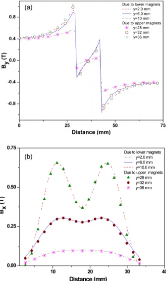
The axial and circumferential components of the magnetic flux density due to the lower and upper magnets in the air gap region are shown in Fig. 5(a) and Fig. 5(b), respectively. The results show that the axial and circum-ferential components of magnetic flux density due to the lower magnet decrease as y increases up to the center of the coil, i.e., 19 mm. The result also shows that the axial and circumferential components of the magnetic flux density due to upper magnets increase as y increases from the center of the coil, i.e., 19 mm.
The axial and circumferential components of the
mag-2 2 1 1 2 1 2 1 1 ( , ) ( )( ) = − −
∫ ∫
R y eff R y wn B K B R y dRdy R R y y 2 1 2 2 6 ( ) = ph − b eff fT E R R B pFig. 5. (Color online) (a) Axial component of the field in the air gap (b) Circumferential component of the field in the air gap.
Fig. 6. (Color online) (a) Axial component of the field in the magnet regions. (a) Circumferential component of the field in magnet regions.
netic flux density due to the lower and upper magnets in the magnet region are shown in Fig. 6(a) and Fig. 6(b), respectively. The results show that the axial and circum-ferential components of the magnetic flux density due to the lower magnet increase as y increases up to the magnet surface. The results also show that the axial and circum-ferential components of the magnetic flux density due to the upper magnet decrease as y increases from the surface of the magnet.
The axial component of the resultant armature reaction at the mean axial position (air gap region) at the rated current for 7 Arms is shown in Fig. 7, by using Equation (17). The armature reaction magnetic field is highest at the edges of the phase band. Also the result shows that the resultant armature reaction field is very small com-pared to the no load magnetic field, and hence can be ignored. The resultant magnetic field is computed by adding the axial and circumferential components of the magnetic field due to the upper and lower magnets. The resultant magnetic field is shown in Fig. 8. The computed resultant magnetic field is at the mean radius and axial height.
The back EMF is computed by using Equation (19). The calculated back EMF is at the mean radius and axial height. The computational time for the back EMF using the analytical method is less than one minute, whereas as it is around 15 hours using 3-D FEA. Thus, the analytical method shows rapid characteristics analysis. The back EMFs computed by using the 2-D analytical method and 3-D FEA are shown in Fig. 9. The back EMFs computed by using both the analytical method and the 3-D FEA are almost equal. The back EMF fundamental harmonic component is 92 % and 90.6 % using the analytical method and 3-D FEA, respectively. Table 2 shows the
summary of the results obtained using the 2-D analytical model and 3-D finite element analysis (FEA). The VTHD is higher for the 3-D FEA analysis because it considers the nonlinear field characteristics.
3. Optimization of the AFPMSG using
2-D Analytical Method
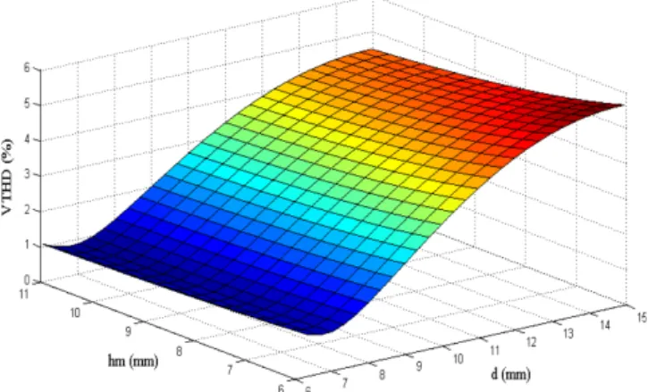
The VTHD varies with the d and hm, as shown in Fig.
Fig. 7. (Color online) Armature reaction field. Fig. 8. (Color online) Resultant magnetic field.
Fig. 9. (Color online) Comparison of back EMF by 2-D ana-lytical method and 3-D FEA of the initial model.
Table 2. 2-D analytical and 3-D FEA performance comparison of the initial model.
Parameters Units 2-D Analytical Method 3-D FEA
back EMF Vpeak 65.7 65.3
10. The VTHD is calculated by computing the back EMF using the 2-D analytical method. It is clear from Fig. 10 that the VTHD increases rapidly as the interpolar separation between the magnet increases. The VTHD also varies with the height of the magnet, but this variation is significantly smaller in comparison.
The optimization of the VTHD % is made with the design variable, interpolar separation, d, and axial height of magnets, hm, while maintaining the back EMF > 65 Vpeak. Figure 11 shows the selected design variable and their optimal values. For the initial model under consideration, hm is equal to 10.0 mm and d is equal to 13.23 mm. An optimal design process employing a developed 2-D analytical method is shown in Fig. 12. The genetic algorithm (GA) and direct search methods are utilized to find the optimized values of the selected design variables and objective functions.
The VTHD has a value of 2.5 % for the initial model by 2-D analytical method. At the optimized values of d and hm provided by the GA and direct search method, the VTHD reduces to 0.39 %. The VTHD % is also computed using 3-D FEA. The result shows that a considerable
reduction in the VTHD is obtained as the result of optimi-zation using the analytical method in the optimized model. The VTHD has a value of 3.15 % and 1.5 % for the initial and optimized models using FEA. The percentage decrease achieved in VTHD is 52.38 % as the result of the optimization using analytical method. Since the 3-D FEA considers the nonlinear characteristics, the VTHD is slightly and consistently higher than the analytical method results.
The back EMF of the optimized model, computed by the 2-D analytical method, is compared with 3-D FEA, as shown in Fig. 13. The result shows that the backs EMF of both the analytical and 3-D FEA are consistent. The analysis of the back EMF waveforms is performed to determine the VTHD and fundamental harmonic compo-nent. Figure 14 shows the comparison of the harmonic components of the initial and the optimized models using 3-D FEA. Since the considered AFPMSG is Y-connected, only the comparison of belt harmonics is considered in this paper. The result shows that the optimized model has an increased fundamental harmonic component. The result
Fig. 10. (Color online) VTHD trend.
Fig. 11. (Color online) Selected design variables and their optimal values.
also shows the reduction in belt harmonics components. Performance comparison of the optimized model using the 2-D analytical method and 3-D FEA is shown in Table 3. The result shows that the back EMF of the optimized model using 2-D analytical method and 3-D FEA are almost the same. The back EMF fundamental harmonic component is 93 % and 92 % using the analy-tical method and 3-D FEA, respectively. Finally, the comparison of the initial design and the optimized design of the AFPMSFG is tabulated in Table 4. The back EMF of the initial and optimized model is almost the same. The percentage decrease in the VTHD is 52.38 % as a result of the optimization. Also the optimized model is more compact in comparison to the initial model.
In order to obtain a load analysis of the AFPMSG's initial and optimized models, a load resistor of 6.8 ohms
Fig. 13. (Color online) Comparison of the back EMF by 2-D analytical method and 3-D FEA for the optimized model.
Fig. 14. (Color online) Belt Harmonics comparison.
Table 3. 2-D analytical and 3-D FEA performance comparison of the optimized model.
Parameters Units 2-D analytical method 3-D FEA
back EMF Vpeak 65.5 65.4
VTHD % 0.39 1.5
Table 4. Comparison of the initial and optimized model. Parameters Units Initial Model Optimized
Model Interpolar separation mm 13.23 6.76714
Height of magnet mm 10.0 8.81239 Axial height of machine mm 46 43.62
back EMF V 65.3 65.4
VTHD % 3.15 1.5
Torque Nm 6.9 7.74
Torque ripple (Tpk2pk) % 45 36
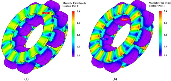
is connected across each phase. The flux density di-stribution of the initial and optimized models under loaded condition is shown in Fig. 15(a) and Fig. 15(b), respectively. The maximum flux density (Bmax) is almost 1.8 T and 2.0 T for the initial and optimized models respectively, which occurs at the rotor back iron. The increased flux density of the optimized model is due to its increased surface area of the magnet due to the decreased interpolar separation as can be seen from the Table 4.
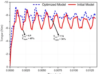
An improvement in the output torque of the optimized model is obtained, as compare to the initial model. A comparison of the output torque of the initial and optimized models is shown in Fig. 16. The output torque of the initial model is 6.9 Nm and that of the optimized model is 7.74 Nm. Furthermore, a reduction in the torque ripple of the optimized model is achieved. The torque ripple of the initial model is 45 % and that of the optimized model it is 36 % by 3D-FEA.
4. Conclusion
This paper presents a 2-D analytical method to compute the back EMF of the coreless dual rotor AFPMSG by solving Maxwell’s equations considering boundary condi-tions. The results of the 2-D analytical method are veri-fied with 3-D FEA. Furthermore, the VTHD % is reduced through optimization with the developed 2-D analytical
method. The VTHD of the initial model is compared with the optimized model using 3-D FEA and results show that the VTHD is 1.5 %, which is a considerable improvement over the previous 3.15 %. Furthermore, the optimal design exhibits reduced torque ripple with higher average output torque, as compare to the initial model. The time saved due the 2-D analytical method proves the advantages of the analytical technique against the time-consuming 3-D FEA method.
References
[1] Asko Parviainen, Ph.D. Thesis, University of Technology Lappeenranta, Finland (2005).
[2] Y. Chen, P. Pillay, and A. Khan, IEEE Trans. Ind. Appl. 41, 6 (2005).
[3] Solmaz Kahourzade, Amin Mahmoudi, and Hew Wooi Ping, Canadian Journal of Electrical and Computation Engineering 37, 1 (2014).
[4] Metin Aydin, Ph.D. Thesis, University of Wisconsin-Madison, (2004).
[5] Chang-Chou Hwang, Ping-Lun Li, Frazier C. Chuang, Cheng-Tsung Liu, and Kuo-Hua Huang, IEEE Trans. Magn. 45, 3 (2009).
[6] W. Fei, P. C. K. Luk and K. Jinupun, IET Electric Power Appl. 4, 9 (2010).
[7] Bing Xia, Jian-Xin Shen, Patrick Chi-Kwong Luk, and Weizhong Fei, IEEE Trans. Ind. Electron. 62, 2 (2015). [8] A. B. Proca, A. Keyhani, and A. EL-Antably, IEEE
Trans. Energy Convers. 18, 3 (2003).
[9] P. Virtic, P. pisek, T. Marcic, M. Hadziselimovic, and B. Stumberger, IEEE Trans. Magn. 44, 11 (2008).
[10] Z. Q. Zhu, D. Howe, E. Bolte, and B. Ackermann, IEEE Trans. Magn. 29, 1 (1993).
[11] E. P. Furlani, Permanent Magnet and Electromechanical Devices, Academic Press, New York (2001) pp. 470-479. [12] J. R. Bumby, R. Martin, M. A. Muller, E. Spooner, N. L. Brown, and B. J. Chalmers, IEEE Proc. Power Appl. 151, 2 (2004).
[13] E. P. Furlani, IEEE Trans. Magn. 30, 5 (1994).
[14] T. F. Chan, L. L. Lai, and S. Xie, IEEE Trans. Energy Convers. 24, 1 (2009).
[15] Yong-min You, Hai Lin, and Byung-il Kwon, JEET 7, 1 (2012).
[16] Richard Martin, Ph.D. Thesis, University of Durham, (2007).
Fig. 16. (Color online) Torque comparison of the initial and optimized model by 3D- FEA.