ESTIMATING THE WAVE HEIGHT OF AZIMUTH TRAVELING OCEAN WAVES BY SAR VELOCITY BUNCHING MODEL
Shunsuke Taniguchi and Kazuo Ouchi
Department of Computer Science, School of Electrical and Computer Engineering,
National Defense Academy, 1-10-20 Hashirimizu, Yokosuka, Kanagawa 239-8686 Japan ( [email protected]) ABSTRACT ... The purpose of this study is to examine the velocity bunching model for ocean wave imagery by SAR (Synthetic Aperture Radar), and to estimate the waveheight of ocean waves propagating in azimuth direction. The SAR data were acquired by the Canadian C-band RADARSAT-1 off the Miura Peninsula in Japan. It has been known theoretically, that for ocean waves propagating in azimuth direction, the image modulation is dominated by velocity bunching with little effect by RCS (Radar Cross Section). Velocity bunching is caused by slant-range velocity components associated with the wave orbital velocity. Because of its highly non-linear nature, the peaks of image intensity may appear at the crests or troughs of waves, double peaks may also occur, and even no image may be produced, depending on the parameters of SAR and ocean waves. Another factor that determines the image modulation is the scene coherence time. The scene coherence time is the average time period over which the backscattered signal maintains a same amplitude and phase, and is proportional to the period during which principal scatters (small-scale waves) keep a same structure. We used the velocity bunching model including the scene coherence time, and estimated the dominant waveheight from the RADARSAT-1 data.
KEY WORDS: SAR, velocity bunching, wave propagation
1. INTRODUCTION
After the launch of SEASAT-SAR in 1978, the study of extracting information on ocean waves by SAR became a notable topic. For ocean waves moving in azimuth direction, the “wave-like” images are often visible, although the backscattering coefficient is nearly constant.
Velocity bunching as a result of orbital motion of ocean waves is considered to attribute this image modulation [1], [2]. However, to date little study has been reported to validate velocity bunching. In the present paper, we examine the velocity bunching effect using RADARSAT-1 data, and estimate the waveheight which is then compared with the JWA (Japan Weather Association) numerical model.
2. VELOCITY BUNCHING 2.1 Principle of Azimuth Image Shift
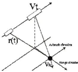
Synthetic aperture technique enables to create high- resolution images in azimuth direction. Figure. 1 shows the SAR geometry where a point scatterer is moving in slant- range direction with the slant-range velocity of vR, V is the platform velocity, r(t) is the slant-range distance between the antenna and scatterer at azimuth time t, and R0 is the reference slant range distance.
The received signal at azimuth time t is given by (1) where k=2π/λ is the wavenumber, λ is wavelength. σ0 is backscatter coefficient. For R0 is large compared with VT, the slant range distance r can be approximated as
Figure 1. Geometry of SAR and a moving scatterer.
(2) When σ0 =1, the received signal can be written as
(3) The image amplitude (point spread function) by cross- correlating equation (3) with a reference signal (complex conjugate of an expected received signal).
(4) The reference signal is weighed by a Gaussian function with the effective synthetic aperture time T. The cross- correlation integral is defined as
(5) where t’ is the azimuth time variable in the image plane.
The point spread function can be obtained by substituting equation (3) and equation (4) into equation (5) as follows.
(6)
where E0 is a constant, X=Vt’ is the azimuth spatial variable in the image plane, and ΔX is the spatial resolution defined as
(7) As can be seen from equation (6), the image of a moving scatterer with slant-range velocity component vr
is displaced in azimuth by distance
(8) This is the basis of the velocity bunching effect in which the slant-range velocity varies in azimuth according to the orbital motion of azimuth traveling waves.
2.2 Velocity Bunching
Small ripples on swell waves that satisfy the Bragg resonant condition are the main scattering elements.
These ripples have up-and-down orbital motion which yields azimuth varying vR. The time-varying ocean waveheight can be expressed as
(9) where h0 is the wave amplitude, k0=2π/L is wavenumber.
ω0=2πv0/L is the angular frequency, L is the wavelength, and v0 is the wave phase velocity. The slant-range velocity component can be expressed as
(10) where q is the incidence angle. Equation (10) shows that the slant-range velocity varies in accordance with the circular function. An exact solution for image intensity can be obtained by substituting equation (10) into equation (2) and by carrying out the convolution integral
(11)
where a(x) is the backscattered amplitude assumed to be constant. Taking into account the scene coherence time or the ripple de-correlation time t0, the mean image intensity can be written as
(12) Mn is n-th order modulation transfer function. Mn can be expressed as
(13) where
(14)
In equation (13), Jn is n-th order Bessel function of 1st kind. ΔX’ in equation (14) is the effective resolution cell degraded by the scene coherent time t0. The de- correlation time is one of the factors which are considered to attribute to the image modulation. The de- correlation time is the average time period over which the backscattered signal maintains a same amplitude and phase, and is proportional to the period during which principal scatterers keep a same structure. Equation (12) is the formula that expresses the image modulation induced by velocity bunching.
This image modulation occurs as a result of densely and sparsely distributed point spread functions in a periodic manner (Figure 2). Because of its highly non-linear nature, the peaks of image intensity may appear at the crests of troughs of waves, double peaks may also occur, and even no image may be produced, depending on the parameters of SAR and ocean waves.
Figure 2. Illustrating the image modulation by velocity bunching in azimuth direction.
3. EXPERIMENTS
Figure 3 shows the grid points overlaid on RADARSAT- 1 image, where the inter-grid distances are approximately 4.6 km in horizontal direction and 5.5 km in vertical direction. The arrows show the wave direction, and the length of the arrows indicates wavelength. The red and blue arrows correspond respectively to the estimates by SAR data and JWA (Japan Weather Association) numerical data, and the numbers under the arrows indicate the significant waveheight by the JWA model.
Comparison of the wavelength, direction and waveheight estimated from the RADARSAT-1 data and those from the JWA model were made as follows.
3.1 Wavelength
Comparison of wavelength was made between SAR data and JWA numerical data to examine the velocity
Figure 3. Grid mesh points overlaid on the RADARSAT- 1 image of the waters of Sagami Bay off the Miura Peninsula (upper). For details, see the text.
bunching model. SAR data were obtained by the C-band RADARSAT-1 SAR, off the Miura Peninsula in Japan as in Figure 3. The specifications of RADARSAT-1 data are listed in Table 1 and those of the JWA numerical model in Table 2.
Table 1. Specification of SAR data
Platform RADARSAT-1
Date 8th July 2000
14:35:53 (UTC)
Mode Fine
Incidence angle 47.79°
Platform velocity 7549.30 m/sec
Altitude 795552.6 m
Wavelength 5.66 cm (C-band)
Image position
Center 35°13’N 139°17’E NW 35°29’N 139°17’E NE 35°24’N 139°51’E SW 35°03’N 139°12’E SE 34°58’N 139°45’E Table 2. Specification of JWA numerical data
Date 8th July 2000
15:00:00 (UTC) Observation place Sagami Bay
The result of comparison is shown in Table 3 for 15 grids labelled as in Figure 3. There appears substantial difference between the two. Even taking into account the fact that the wave forecast by JWA is generally made per large sea area, the wavelength averaged over all grid points in SAR data is 380 m, while that by JWA model is 525 m. The average SAR data underestimate the wavelength by 38.2 % in comparison with the JWA data.
If the error estimate, 100 (LSAR-LJWA)/LSAR is used for individual grids, the accuracy averaged over all 15 grids
Table 3. Comparison of wavelength between SAR data and JWA data
SAR data [m] JWA data [m] 8 378 593
1 567 394 9 401 575
2 314 467 10 378 599
3 567 451 11 275 1014
4 444 551 12 321 375
5 444 557 13 283 375
6 444 551 14 298 399
7 298 569 15 283 399
is 47.6% of underestimation.
If the depth correction [2] was applied to JWA data, slightly lower 47.3 % error was obtained, but it is within a random error, i.e., virtually no improvement. The reason may well be associated with the JWA model.
3.2 Wave Direction
Wave direction was estimated by applying weighed- cross-correlation [3] to the sub-aperture SAR images.
The results are shown in Table 4. The accuracy was estimated according to equation (15).
(15) The result showed fairly good agreement with the estimation error of 16.6°.
Table 4. Comparison of Wave direction between SAR data and JWA data
SAR data[deg] JWA data[deg] 8 141 131
1 141 112 9 180 142
2 107 137 10 141 144
3 141 133 11 127 091
4 152 141 12 133 127
5 152 140 13 141 127
6 152 140 14 164 128
7 118 138 15 141 128
3.3 Waveheight
The basic idea of waveheight estimation is first to assume the de-correlation time from the SAR image contrast combined with theoretical expression, and by comparing with the JWA waveheight. A theoretical model is then formulated based on Equation (12). There are two unknowns (waveheight and de-correlation time) to determine the theoretical image contrast, and one known experimental parameter. Thus, unless the de- correlation time is known, the waveheight cannot be deduced from the SAR data.
In our approach, the de-correlation time is first estimated from best-fitted waveheight between the image contrast and JWA data. Once the de-correlation time t0 is
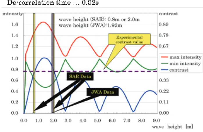
known, the waveheight in other scenes can be estimated under the condition that the same de-correlation time holds. This condition is very important, but it has been reported that the de-correlation time at L-band is around 0.02 s [5].
The SAR images of ocean waves travelling predominantly in azimuth direction were extracted, and the median contrast value was calculated. At the same time, the theoretical image contrast was computed for different t0 and waveheight h0. The best-fitted de- correlation time is then sought, which yields the same waveheight between the theory and the JWA data. Since the de-correlation time is known, we can formulate the image modulation in Equation (12), which can be used to estimate the waveheight in other areas, provided that, of course, the de-correlation time is the same in the other areas. From the experiment, we obtained the similar waveheight estimation between the theory and JWA data, when t0=0.02 s as in Figure 4. Comparison of waveheight between SAR data and JWA data is listed in Table 4.
Figure 4. Comparison between SAR image intensity and theoretical image intensity
Table 4. Comparison of waveheight between SAR data and JWA data in [m] for different de-correlation times in [s].
De-correlation time
h0 from SAR data h0 from JWA data 0.02 0.8,2.0
1.92 0.05 0.4,2.8,3.3,5.1,
5.8,6.8
0.10 0.3,3.1,5.5,7.7 8.1
0.15 0.3,5.6,7.9 0.20 0.4,8.0
4. CONCLUSIONS 4.1 Conclusion
Attempt has been made to estimate the waveheight of azimuth travelling using the velocity bunching model. In order to test the theory, RADARSAT-1 data and JWA data were used. The result showed that agreement on the
wavelength was not satisfactory despite the water depth correction, good agreement was obtained on the wave direction, and good agreement was obtained on the waveheight at the de-correlation time of 0.02 sec. These results can be used to improve the wave forecast numerical model.
References:
[1] Werner Alpers and Clifford L. Rufenach, “The effect of orbital motion on synthetic aperture radar imagery of ocean waves,” IEEE Trans, Antennas Propagat., vol.27, pp.685-690, 1979.
[2] Kazuo Ouchi, Donald A. Burridge, “Resolution of a controversy surrounding the focusing mechanisms of synthetic aperture radar images of ocean waves”. IEEE Trans.
Geosci. Remote Sensing, vol. 32, pp. 1004-1016, 1994.
[3] Hisashi Mitsuyasu. Physics of Ocean Waves (in Japanese).
Iwanami Press Publishing Co., 2002.
[4] Kazuo Ouchi, Shoji Maedoi, and Hisashi Mitsuyasu,
“Determination of ocean wave propagation direction by split- look processing using JERS-1 SAR data”. IEEE Trans.
Geosci. Remote Sens., vol. 37, pp. 849-855, 1999.
[5] M.J.Tucker, “The decorrelation time of microwave radar echoes from the sea surface,” Int J. Remote Sens., vol 6, pp.1075-1089, 1985